Before reading this blog, I recommend you to read the first 4 parts of this blog series. Available below:
Do geopolitical risks raise or lower inflation? Part V
Pooled versus unit-by-unit estimators
In the previous posts, I focused on how geopolitical risk shocks affect inflation, output, and the main transmission channels in the long historical panel assembled by Caldara, Conlisk, Iacoviello, and Penn. A natural question remains: are those results driven by the pooling assumption, or do they survive once we allow countries to respond differently to geopolitical shocks?
This is exactly the purpose of Figure 7 in the Journal of International Economics paper. The figure compares the baseline pooled estimator with 2 alternative estimators built from country-by-country VARs. In my view, this is one of the most important figures in the paper, because it addresses a central econometric concern: the possibility that the average effects reported earlier are masking substantial dynamic heterogeneity across countries.
The answer is reassuring. The inflationary effects of geopolitical risk do not disappear once one moves away from the pooled panel VAR. They remain visible, economically meaningful, and qualitatively consistent with the baseline results.
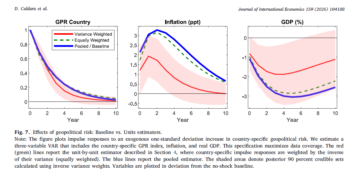
The figure reports impulse responses to an exogenous 1-standard-deviation increase in country-specific geopolitical risk. The specification is intentionally parsimonious: a 3-variable VAR including the country-specific GPR index, inflation, and real GDP. This choice is not a weakness. On the contrary, it maximizes country coverage and makes the comparison between estimators cleaner.
The blue line is the pooled estimator, which imposes common dynamics across countries after demeaning the variables at the country level. The red line is the inverse-variance weighted aggregation of country-specific impulse responses. The green dashed line is the equally weighted aggregation, where each country contributes the same weight regardless of the precision of its estimated response. The shaded area is the 90 percent credible set around the inverse-variance weighted estimator.
This setup is useful because the 3 estimators answer slightly different questions. The pooled estimator is efficient if the homogeneity restriction is approximately valid. The equally weighted estimator is closer to the average country response in a literal sense, because each country counts the same. The inverse-variance weighted estimator gives more weight to countries whose responses are estimated more precisely. If the substantive conclusions are similar across these approaches, confidence in the results increases considerably.
That is precisely what happens here.
The first panel, for country-specific geopolitical risk itself, shows that the shock is highly persistent under all 3 estimators. The red, green, and blue lines all decline gradually from the impact response, with only moderate differences in persistence. This is an important starting point, because it confirms that the dynamic profile of the identified shock is not an artifact of the pooled procedure.
The second panel is the one that matters most for the paper’s main claim. Inflation rises persistently after a geopolitical risk shock under all 3 estimators. The pooled response is the strongest, peaking a little above 3 percentage points. The equally weighted response is also large and follows a very similar shape, although at a slightly lower level. The inverse-variance weighted response is more muted, but it remains clearly positive and persistent. This ranking is informative. It suggests that countries with larger inflation responses also tend to have noisier estimates, so that they receive less weight in the inverse-variance aggregation. But the basic message is unchanged: the inflationary effect is not a fragile feature of the pooled estimator.
The third panel shows that GDP falls after the shock under all 3 estimators. Once again, the pooled and equally weighted estimates are quite close, while the inverse-variance weighted response is somewhat less negative. But the sign is consistent throughout. This matters a great deal for interpretation. If geopolitical risk were mainly operating through demand compression, one might expect inflation to fall together with output, or at least to display weaker inflationary effects. Instead, the joint pattern of higher inflation and lower GDP is much more consistent with a supply-side disturbance, or at least with a shock in which supply effects dominate.
This is one of the main strengths of Figure 7. It does not merely say that the pooled model is “robust.” It shows that the central macroeconomic pattern of the paper survives when one moves to an estimator that is explicitly designed to tolerate heterogeneity across countries.
There is also a deeper econometric lesson here. In macro panel VAR work, pooling is always tempting because it improves precision and allows one to use more of the available data. But pooling can be misleading if the true data-generating process differs substantially across units. Figure 7 addresses this issue directly. The comparison between pooled and unit-by-unit estimators does not reveal a contradiction. Rather, it reveals a difference of magnitude, not of sign or mechanism. That is the kind of robustness result one wants to see.
From a substantive perspective, the figure also helps clarify how to read the earlier results. The pooled estimator appears to provide a good summary of the average dynamics in the sample. The equally weighted estimator, which is arguably the most literal measure of the “average country,” is remarkably close to it. The inverse-variance weighted estimator is smaller, but it still points in the same direction. Taken together, these responses suggest that the inflationary consequences of geopolitical risk are broad-based rather than driven by just a handful of countries.
This is especially important in a long historical sample mixing advanced and emerging economies, wartime and peacetime episodes, and very different institutional settings. One could easily have imagined a much less stable pattern. Instead, the figure suggests that the result is surprisingly general: geopolitical risk tends to raise inflation and reduce output, even once we stop imposing common dynamics mechanically.
In replication terms, this figure is also interesting because it is more delicate than the earlier pooled figures. Once one estimates country-by-country VARs, aggregation choices matter a lot. One has to decide how to weight the country responses, how to construct the credible sets, and how to scale the GDP response so that it is expressed in percent rather than raw decimal units. Small coding mistakes can flatten the GDP response or make the band disappear visually. But once these details are handled properly, the logic of the figure becomes very transparent.
My overall reading of Figure 7 is therefore straightforward. The main conclusion of the paper survives a serious heterogeneity check. Geopolitical risk is inflationary on average, and it is also contractionary for real activity. The exact magnitude depends on how one aggregates country responses, but the qualitative message is stable. That makes the earlier pooled evidence much more persuasive.
In other words, the inflationary consequences of geopolitical risk are not just a pooled-panel artifact. They remain visible when countries are first allowed to speak with their own voice, and only then aggregated.
That is why Figure 7 deserves to be read not as a peripheral robustness exercise, but as one of the core figures of the paper.f robustness that gives the earlier figures more weight.
Conclusion
Figure 7 shows that the core result of Caldara et al. is not driven by the homogeneity assumption of the pooled panel VAR. Whether one uses the pooled estimator, an equally weighted average of country-specific VARs, or an inverse-variance weighted aggregation, geopolitical risk still tends to raise inflation and lower GDP. This is a strong and reassuring robustness result.
References
Caldara, D., Conlisk, S., Iacoviello, M., & Penn, M. (2026). Do geopolitical risks raise or lower inflation? Journal of International Economics, 104188.
Figure 7 code
version 18.0

capture log close _f7
log using "$JIE_LOG/24_figure7_units_estimators.log", replace text ///
    name(_f7)

use "$JIE_DER/annual_panel.dta", clear
sort country_id year
xtset country_id year

local yraw ///
    gpr_country ///
    inflation_ppt ///
    gdp_pct

egen __rowmiss_f7 = rowmiss(`yraw')
gen byte sample_f7 = (__rowmiss_f7 == 0)
drop __rowmiss_f7

count if sample_f7
display as text "Figure 7 raw complete-case observations: " r(N)

foreach v of local yraw {
    by country_id: egen mean_`v'_f7 = mean(cond(sample_f7, `v', .))
    gen dm_`v'_f7 = cond(sample_f7, `v' - mean_`v'_f7, .)
}

local ydm
foreach v of local yraw {
    local ydm `ydm' dm_`v'_f7
}

mata: jie_bvar_pooled_summary( ///
    "`ydm'", "country_id", "year", "sample_f7", ///
    $JIE_P, $JIE_H, $JIE_NDRAWS, 1, 1, ///
    "F7P_Q05", "F7P_Q50", "F7P_Q95", ///
    "F7P_MEAN", "F7P_VAR", "F7P_Neff" ///
)

display as text "Figure 7 lag-valid pooled rows: " ///
    %9.0g scalar(F7P_Neff)

bys country_id: egen T_f7 = total(sample_f7)
egen tag_country = tag(country_id)

display as text ///
    "Figure 7 countries retained by the $JIE_MINOBS-observation rule:"
levelsof country if tag_country & T_f7 >= $JIE_MINOBS, local(keep_f7)
local nkeep_f7 : word count `keep_f7'
display as text "Figure 7 included countries: `nkeep_f7'"

display as text ///
    "Figure 7 countries excluded by the $JIE_MINOBS-observation rule:"
levelsof country if tag_country & T_f7 < $JIE_MINOBS, local(drop_f7)
local ndrop_f7 : word count `drop_f7'
display as text "Figure 7 excluded countries: `ndrop_f7'"

mata: jie_bvar_units_aggregate( ///
    "`yraw'", "country_id", "year", "sample_f7", ///
    $JIE_MINOBS, $JIE_P, $JIE_H, $JIE_NDRAWS, 1, 1, ///
    "F7_IVW", "F7_EW", "F7_B05", "F7_B95", "F7_Ncountry" ///
)

display as text "Figure 7 countries used in aggregation: " ///
    %9.0g scalar(F7_Ncountry)

local cnP50
local cnIVW
local cnEW
local cnB05
local cnB95
foreach v of local yraw {
    local cnP50 `cnP50' pooled_q50_`v'
    local cnIVW `cnIVW' ivw_`v'
    local cnEW  `cnEW'  ew_`v'
    local cnB05 `cnB05' band_q05_`v'
    local cnB95 `cnB95' band_q95_`v'
}

matrix colnames F7P_Q50 = `cnP50'
matrix colnames F7_IVW  = `cnIVW'
matrix colnames F7_EW   = `cnEW'
matrix colnames F7_B05  = `cnB05'
matrix colnames F7_B95  = `cnB95'

preserve
clear
set obs `= $JIE_H + 1'
gen horizon = _n - 1

svmat double F7P_Q50, names(col)
svmat double F7_IVW,  names(col)
svmat double F7_EW,   names(col)
svmat double F7_B05,  names(col)
svmat double F7_B95,  names(col)

replace pooled_q50_gdp_pct = 100 * pooled_q50_gdp_pct
replace ivw_gdp_pct        = 100 * ivw_gdp_pct
replace ew_gdp_pct         = 100 * ew_gdp_pct
replace band_q05_gdp_pct   = 100 * band_q05_gdp_pct
replace band_q95_gdp_pct   = 100 * band_q95_gdp_pct

save "$JIE_DER/fig7_irf.dta", replace
export delimited using "$JIE_DER/fig7_irf.csv", replace

local bandcol "pink"
local pcol    "blue"
local ivwcol  "red"
local ewcol   "forest_green"

twoway ///
    rarea band_q05_gpr_country band_q95_gpr_country horizon, ///
        color(`bandcol'%25) lcolor(`bandcol'%0) || ///
    line ivw_gpr_country horizon, ///
        lcolor(`ivwcol') lwidth(medthick) || ///
    line ew_gpr_country horizon, ///
        lcolor(`ewcol') lwidth(medthick) ///
        lpattern(shortdash) || ///
    line pooled_q50_gpr_country horizon, ///
        lcolor(`pcol') lwidth(thick) || ///
    , ///
    title("GPR Country", size(medium) color(black)) ///
    yline(0, lcolor(black%35) lwidth(vthin)) ///
    xtitle("Year", size(medsmall)) ///
    ytitle("") ///
    xlabel(0(2)$JIE_H, labsize(medsmall) nogrid) ///
    yscale(range(-0.08 1.05)) ///
    ylabel(0 .2 .4 .6 .8 1, nogrid labsize(medsmall)) ///
    legend(order(2 "Variance Weighted" ///
                 3 "Equally Weighted" ///
                 4 "Pooled / Baseline") ///
           rows(3) size(small) ring(0) pos(2) ///
           region(lcolor(black) fcolor(white))) ///
    graphregion(color(white) margin(small)) ///
    plotregion(color(white) margin(tiny)) ///
    name(gr7_gpr_country, replace)

twoway ///
    rarea band_q05_inflation_ppt band_q95_inflation_ppt horizon, ///
        color(`bandcol'%25) lcolor(`bandcol'%0) || ///
    line ivw_inflation_ppt horizon, ///
        lcolor(`ivwcol') lwidth(medthick) || ///
    line ew_inflation_ppt horizon, ///
        lcolor(`ewcol') lwidth(medthick) ///
        lpattern(shortdash) || ///
    line pooled_q50_inflation_ppt horizon, ///
        lcolor(`pcol') lwidth(thick) || ///
    , ///
    title("Inflation (ppt)", size(medium) color(black)) ///
    yline(0, lcolor(black%35) lwidth(vthin)) ///
    xtitle("Year", size(medsmall)) ///
    ytitle("") ///
    xlabel(0(2)$JIE_H, labsize(medsmall) nogrid) ///
    yscale(range(-0.7 3.4)) ///
    ylabel(-.5 0 .5 1 1.5 2 2.5 3, ///
        nogrid labsize(medsmall)) ///
    legend(off) ///
    graphregion(color(white) margin(small)) ///
    plotregion(color(white) margin(tiny)) ///
    name(gr7_inflation_ppt, replace)

twoway ///
    rarea band_q05_gdp_pct band_q95_gdp_pct horizon, ///
        color(`bandcol'%25) lcolor(`bandcol'%0) || ///
    line ivw_gdp_pct horizon, ///
        lcolor(`ivwcol') lwidth(medthick) || ///
    line ew_gdp_pct horizon, ///
        lcolor(`ewcol') lwidth(medthick) ///
        lpattern(shortdash) || ///
    line pooled_q50_gdp_pct horizon, ///
        lcolor(`pcol') lwidth(thick) || ///
    , ///
    title("GDP (%)", size(medium) color(black)) ///
    yline(0, lcolor(black%35) lwidth(vthin)) ///
    xtitle("Year", size(medsmall)) ///
    ytitle("") ///
    xlabel(0(2)$JIE_H, labsize(medsmall) nogrid) ///
    yscale(range(-3.6 0.6)) ///
    ylabel(-3 -2 -1 0, nogrid labsize(medsmall)) ///
    legend(off) ///
    graphregion(color(white) margin(small)) ///
    plotregion(color(white) margin(tiny)) ///
    name(gr7_gdp_pct, replace)

graph combine ///
    gr7_gpr_country ///
    gr7_inflation_ppt ///
    gr7_gdp_pct, ///
    cols(3) ///
    imargin(1 1 1 1) ///
    graphregion(color(white) margin(2 2 2 2)) ///
    name(fig7_combined, replace)

graph save "$JIE_FIG/figure7_units_estimators_journalstyle.gph", replace
graph export "$JIE_FIG/figure7_units_estimators_journalstyle.png", ///
    width(2400) replace

restore
drop tag_country T_f7
log close _f7