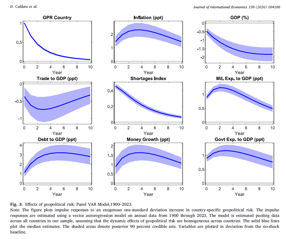
Today, I will start a series of blog to replicate the Figures of recent research on the macroeconomic effects of geopolitical risk. In “Do geopolitical risks raise or lower inflation?,” Caldara, Conlisk, Iacoviello, and Penn (CCIP, hereafter) ask a very important question. The Figure 3 in CCIP shows that after an adverse country-specific geopolitical risk shock, inflation rises, GDP falls, trade contracts, shortages increase, military spending rises, debt rises, money growth rises, and government spending increases. In other words, geopolitical risk looks inflationary and contractionary at the same time. That is precisely what makes the figure so interesting for macroeconomists. The paper estimates these responses in a pooled panel VAR on annual data from 1900 through 2023 and reports posterior median impulse responses together with 90 percent credible sets.
I wanted to see how closely this figure could be replicated in a transparent Stata/Mata workflow. The answer is: quite closely.
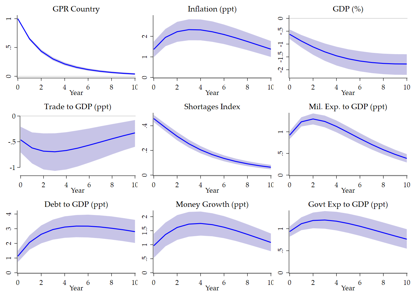
The final replication matches the published figure well in the dimensions that matter most. Country GPR declines monotonically after the shock. Inflation follows a hump-shaped response. GDP declines persistently. Trade falls and only partially recovers. Shortages fade gradually from an elevated level. Military expenditures, debt, money growth, and government spending all increase after the shock. These are the core dynamic patterns in the published figure, and they all emerge clearly in the replication. In the following, I include, first, Figure 3 in the paper and, then, my replication using Stata/Mata abilities:
Now, my replication with the pooled panel Bayesian VAR:
The paper’s baseline specification is a pooled panel VAR that assumes homogeneous dynamic effects across countries, estimated on annual data from 1900 through 2023. The authors state that the model is estimated with 1 lag in the baseline, with a Bayesian VAR using an uninformative Jeffreys prior and 5000 Gibbs-sampler draws from the posterior distribution. The plotted solid lines are posterior medians, and the shaded areas are posterior 90 percent credible sets.
My replication follows the same broad logic. I start from the annual panel, keep the 9 variables used in Figure 3, demean them by country to account for country fixed effects, estimate a pooled dynamic system, and then compute impulse responses to a 1-standard-deviation increase in country-specific geopolitical risk. The result is a custom pooled panel Bayesian VAR in Stata/Mata designed to reproduce the same economic object as the published figure.
That last sentence is important. The replication reproduces the economic object very well, but it should not automatically be interpreted as a literal line-by-line reproduction of the exact Bayesian code used in the paper. The published paper relies on a Jeffreys-prior Bayesian VAR with posterior simulation via Gibbs sampling, implemented using the Canova-Ferroni toolbox. My Mata function is written from scratch and is meant to be transparent and pedagogical. It delivers posterior-style summaries and credible sets, but its internal simulation mechanics are not necessarily identical to the original toolbox.
Why does this matter? Because in replication work there are different notions of success. A first notion is qualitative replication: do the responses have the same signs, shapes, and economic interpretation? Here the answer is clearly yes. A second notion is quantitative replication: are the peak and long-horizon effects of similar magnitude? Again, yes. A third notion is algorithmic identity: did we use the same prior, the same sampling procedure, and the same exact treatment of the covariance matrix and posterior draws? Here the answer is more cautious. The custom Mata function is best viewed as a pedagogical Bayesian pooled panel VAR that recovers the same substantive dynamics, not necessarily the exact original Gibbs simulator.
In practice, this distinction showed up mostly in the confidence bands and in a few graphical details. The median responses were close rather quickly. The harder parts were mundane but revealing: getting the GDP units right, making sure trade-axis labels displayed properly, and matching the visual style of the journal figure. At one point, the GDP response looked almost flat simply because the stored IRFs were still in decimal units rather than in percent. Multiplying the GDP impulse responses by 100 resolved the issue immediately and aligned that panel with the paper. The trade panel required explicit y-axis labels to avoid clipping in the combined graph. Once those details were corrected, the replication became visually convincing.
Substantively, the exercise confirms the central macroeconomic message of the paper. The joint behavior of inflation and GDP suggests a stagflationary pattern. Inflation rises while output declines. Trade falls, shortages remain elevated, and policy variables respond in an expansionary direction. The paper interprets this combination as evidence that the supply-side effects of geopolitical risk dominate, even though demand and policy channels also move. The replication supports exactly that reading.
This is also a useful reminder that Figure 3 is a pooled-dynamics object, not a mean-group average of country-by-country responses. The paper is explicit that the baseline pools data across countries and assumes common dynamics in the baseline specification, before later exploring heterogeneity with alternative estimators. That distinction matters because it explains why a single pooled panel VAR can summarize such a long historical sample so compactly.
So what is the value of reproducing this figure in custom Mata code? For me, it is mainly pedagogical. It makes the econometrics more transparent. Once one strips away the journal layout and the original toolbox, Figure 3 becomes easier to understand: a pooled dynamic system, a recursive identification with country GPR ordered first, a Bayesian posterior summary, and a set of impulse responses that trace how geopolitical shocks propagate through inflation, activity, trade, shortages, and fiscal-monetary variables. Seen this way, the figure is not a black box. It is a coherent empirical object that can be reconstructed, studied, and taught.
The bottom line is simple. Figure 3 is replicable in a meaningful sense. A carefully written pooled panel Bayesian VAR in Stata/Mata can recover the same main dynamics and deliver a figure that is very close to the published one. The remaining differences are small and mostly concern graphical styling and the exact geometry of the credible sets. That is a reassuring result. It suggests that the paper’s core message is not an artifact of inaccessible code or an idiosyncratic plotting routine. It is a robust feature of the underlying dynamic system.
Short code appendix
The core logic of the replication is simple.
First, define the 9 variables in the annual panel and keep complete cases for the figure:
local yraw ///
    gpr_country inflation_ppt gdp_pct trade_to_gdp_ppt ///
    shortages_index milit_exp_to_gdp_ppt debt_to_gdp_ppt ///
    money_growth_ppt govt_exp_to_gdp_pptegen __rowmiss_f3 = rowmiss(`yraw')
gen byte sample_f3 = (__rowmiss_f3 == 0)
Second, demean each variable by country:
foreach v of local yraw {
    by country_id: egen mean_`v'_f3 = mean(cond(sample_f3, `v', .))
    gen dm_`v'_f3 = cond(sample_f3, `v' - mean_`v'_f3, .)
}
Third, pass the demeaned variables to the Mata routine that computes the pooled panel Bayesian VAR summaries:
mata: jie_bvar_pooled_summary( ///
    "`ydm'", "country_id", "year", "sample_f3", ///
    $JIE_P, $JIE_H, $JIE_NDRAWS, 1, 1, ///
    "F3_Q05", "F3_Q50", "F3_Q95", ///
    "F3_MEAN", "F3_VAR", "F3_Neff" ///
)
Fourth, reshape the output into Stata variables, rescale GDP from decimals to percent, and plot posterior medians with credible bands:
svmat double F3_Q05, names(col)
svmat double F3_Q50, names(col)
svmat double F3_Q95, names(col)replace q05_gdp_pct = 100 * q05_gdp_pct
replace q50_gdp_pct = 100 * q50_gdp_pct
replace q95_gdp_pct = 100 * q95_gdp_pct
The main lesson is that once the data treatment, pooling logic, and scaling are handled carefully, the figure falls into place.
References
Caldara, D., Conlisk, S., Iacoviello, M., & Penn, M. (2025). Do geopolitical risks raise or lower inflation?. Journal of International Economics, 104188.
Code appendix
Mata Bayesian VAR
The Mata code does not use:
- burn-in,
- thinning,
- multiple chains,
- convergence diagnostics.
It simply generates 5000 posterior draws from the conjugate posterior and uses all 5000 to compute the posterior summaries.
So the implementation is a direct conjugate posterior simulator, not an MCMC design where burn-in and thinning are needed in the usual sense.
Exact structure of the Bayesian routine
The Mata routine does the following.
1. Build the stacked panel regression
The data are reorganized into the multivariate regression:
where:
- is the matrix of current observations of the endogenous variables,
- contains the lagged endogenous variables and a constant,
- is the coefficient matrix,
- is the matrix of reduced-form residuals.
For a VAR with variables and , the regressor count is:
because the code includes:
- 1 constant,
- 1 lag of each of the endogenous variables.
The effective sample size used inside the posterior formulas is the number of valid stacked panel transitions after checking:
- same country,
- consecutive year,
- nonmissing current and lagged observations.
2. Prior/posterior setup
The code uses an uninformative Jeffreys-type prior, implemented through the standard conjugate multivariate-regression posterior.
Conditional on , the posterior for is Gaussian.
Conditional on , the posterior for is inverse-Wishart.
The key posterior quantities are:
- OLS coefficient estimate:
- residual matrix:
- sum of squared residuals:
- posterior degrees of freedom:
where:
- is the effective number of rows in the stacked regression,
- is the number of regressors per equation.
The code explicitly checks that:
otherwise it stops with an error.
Exact draw mechanics
For each of the 5000 draws, the code does this:
Step 1. Draw
This is implemented in Mata by:
- symmetrizing ,
- drawing a Wishart random matrix for ,
- inverting it to obtain an inverse-Wishart draw.
Step 2. Draw
The code computes:
and draws
where:
- is the Cholesky factor of ,
- is the Cholesky factor of ,
- is an matrix of iid standard normals.
So each draw of is centered at the multivariate OLS estimate and scaled by both regressor uncertainty and covariance uncertainty.
IRF computation
For each draw , the code computes orthogonalized IRFs.
Companion form
The code builds the VAR companion matrix from the lag coefficients in .
With , this is especially simple: the companion matrix is just the first-lag coefficient block.
Identification
The code uses recursive identification via the Cholesky factor of :
with lower triangular.
Scaling
The code normalizes the shock by the contemporaneous response of the selected scale variable.
Concretely, it sets the initial state to the selected Cholesky shock column, then divides the whole IRF path by:
If that scale is numerically too close to zero, it sets the scale to 1.
So the reported IRFs are normalized relative to the selected impact response.
Posterior summaries stored
For pooled figures, after the 5000 draws the code stores:
- q05
- q50
- q95
- posterior mean
- posterior variance
for every response variable and every horizon.
So the reported intervals are:
- median = 50th percentile
- 90 percent credible set = 5th to 95th percentile
version 18.0

mata:
mata clear

real scalar function jie__quantile(real colvector x, real scalar p)
{
    real scalar n, pos, lo, hi, w
    x = sort(x, 1)
    n = rows(x)
    if (n == 0) return(.)
    if (n == 1) return(x[1])
    pos = 1 + (n - 1) * p
    lo  = floor(pos)
    hi  = ceil(pos)
    if (lo == hi) return(x[lo])
    w = pos - lo
    return((1 - w) * x[lo] + w * x[hi])
}

real rowvector function jie__colmeans(real matrix X)
{
    return(colsum(X) / rows(X))
}

real rowvector function jie__colvars(real matrix X)
{
    real rowvector mu
    if (rows(X) <= 1) return(J(1, cols(X), .))
    mu = jie__colmeans(X)
    return(colsum((X :- mu) :^ 2) / (rows(X) - 1))
}

real matrix function jie__build_xy(real matrix Yall, real colvector id, real colvector year, real colvector sample, real scalar p)
{
    real scalar N, K, nvalid, t, l, ok, r, c
    real matrix ZX

    N = rows(Yall)
    K = cols(Yall)

    nvalid = 0
    for (t = p + 1; t <= N; t++) {
        ok = (sample[t] == 1)
        if (ok) {
            for (l = 1; l <= p; l++) {
                if (id[t-l] != id[t] | (year[t] - year[t-l]) != l | sample[t-l] != 1) {
                    ok = 0
                    break
                }
            }
        }
        nvalid = nvalid + ok
    }

    ZX = J(nvalid, K + K * p + 1, .)
    r = 1
    for (t = p + 1; t <= N; t++) {
        ok = (sample[t] == 1)
        if (ok) {
            for (l = 1; l <= p; l++) {
                if (id[t-l] != id[t] | (year[t] - year[t-l]) != l | sample[t-l] != 1) {
                    ok = 0
                    break
                }
            }
        }
        if (ok) {
            ZX[r, 1..K] = Yall[t, .]
            c = K + 1
            for (l = 1; l <= p; l++) {
                ZX[r, c..(c + K - 1)] = Yall[t-l, .]
                c = c + K
            }
            ZX[r, cols(ZX)] = 1
            r = r + 1
        }
    }

    return(ZX)
}

real matrix function jie__rwishart(real matrix V, real scalar df)
{
    real scalar K, i
    real matrix A, C

    K = rows(V)
    A = J(K, K, 0)

    for (i = 1; i <= K; i++) {
        A[i, i] = sqrt(rchi2(1, 1, df - i + 1))
        if (i < K) {
            A[(i+1)..K, i] = rnormal(K - i, 1, 0, 1)
        }
    }

    C = cholesky(V)
    return(C * A * A' * C')
}

real matrix function jie__riwishart(real matrix S, real scalar df)
{
    real matrix Winv
    S = 0.5 :* (S + S')
    Winv = jie__rwishart(invsym(S), df)
    return(invsym(Winv))
}

real matrix function jie__companion(real matrix B, real scalar K, real scalar p)
{
    real scalar l
    real matrix F

    F = J(K * p, K * p, 0)
    for (l = 1; l <= p; l++) {
        F[1..K, ((l-1)*K + 1)..(l*K)] = B[((l-1)*K + 1)..(l*K), .]'
    }
    if (p > 1) {
        F[(K+1)..(K*p), 1..(K*(p-1))] = I(K * (p-1))
    }

    return(F)
}

real matrix function jie__oirf(real matrix B, real matrix Sigma, real scalar K, real scalar p, real scalar H, real scalar shock_idx, real scalar scale_idx)
{
    real scalar h, scale
    real matrix F, P, irf
    real colvector state

    F = jie__companion(B, K, p)
    P = cholesky(0.5 :* (Sigma + Sigma'))

    state = J(K * p, 1, 0)
    state[1..K, 1] = P[, shock_idx]

    scale = state[scale_idx, 1]
    if (abs(scale) < 1e-12) scale = 1

    irf = J(H + 1, K, .)
    irf[1, .] = (state[1..K, 1] :/ scale)'

    for (h = 1; h <= H; h++) {
        state = F * state
        irf[h + 1, .] = (state[1..K, 1] :/ scale)'
    }

    return(irf)
}

real matrix function jie__bvar_draws_from_xy(real matrix Y, real matrix X, real scalar p, real scalar H, real scalar ndraws, real scalar shock_idx, real scalar scale_idx)
{
    real scalar T, K, m, nu, d, h, j, idx
    real matrix XtX, Vb, Bhat, E, S, Cb, Sigma, Cs, Z, B, irf, draws

    T = rows(Y)
    K = cols(Y)
    m = cols(X)
    nu = T - m

    if (T <= m | nu <= K - 1) {
        errprintf("Not enough effective observations for the Jeffreys-prior posterior.\n")
        exit(3499)
    }

    XtX = quadcross(X, X)
    Vb  = invsym(XtX)
    Bhat = Vb * quadcross(X, Y)
    E = Y - X * Bhat
    S = quadcross(E, E)
    S = 0.5 :* (S + S')

    Cb = cholesky(Vb)

    draws = J(ndraws, (H + 1) * K, .)

    for (d = 1; d <= ndraws; d++) {
        Sigma = jie__riwishart(S, nu)
        Cs = cholesky(0.5 :* (Sigma + Sigma'))
        Z  = rnormal(m, K, 0, 1)
        B  = Bhat + Cb * Z * Cs'
        irf = jie__oirf(B, Sigma, K, p, H, shock_idx, scale_idx)

        idx = 1
        for (h = 1; h <= H + 1; h++) {
            for (j = 1; j <= K; j++) {
                draws[d, idx] = irf[h, j]
                idx = idx + 1
            }
        }
    }

    return(draws)
}

void function jie__summarize_draws(real matrix draws, real scalar H, real scalar K, string scalar mat_q05, string scalar mat_q50, string scalar mat_q95, string scalar mat_mean, string scalar mat_var)
{
    real scalar h, j, idx
    real rowvector mu, va
    real matrix q05, q50, q95, meanm, varm

    q05   = J(H + 1, K, .)
    q50   = J(H + 1, K, .)
    q95   = J(H + 1, K, .)
    meanm = J(H + 1, K, .)
    varm  = J(H + 1, K, .)

    mu = jie__colmeans(draws)
    va = jie__colvars(draws)

    idx = 1
    for (h = 1; h <= H + 1; h++) {
        for (j = 1; j <= K; j++) {
            q05[h, j]   = jie__quantile(draws[, idx], 0.05)
            q50[h, j]   = jie__quantile(draws[, idx], 0.50)
            q95[h, j]   = jie__quantile(draws[, idx], 0.95)
            meanm[h, j] = mu[idx]
            varm[h, j]  = va[idx]
            idx = idx + 1
        }
    }

    st_matrix(mat_q05, q05)
    st_matrix(mat_q50, q50)
    st_matrix(mat_q95, q95)
    st_matrix(mat_mean, meanm)
    st_matrix(mat_var, varm)
}

void function jie_bvar_pooled_summary(string scalar yvars, string scalar panelvar, string scalar timevar, string scalar samplevar, real scalar p, real scalar H, real scalar ndraws, real scalar shock_idx, real scalar scale_idx, string scalar mat_q05, string scalar mat_q50, string scalar mat_q95, string scalar mat_mean, string scalar mat_var, string scalar scalar_neff)
{
    string rowvector vars
    real matrix Yall, ZX, Y, X, draws
    real colvector id, year, sample
    real scalar K

    vars   = tokens(yvars)
    Yall   = st_data(., vars)
    id     = st_data(., panelvar)
    year   = st_data(., timevar)
    sample = st_data(., samplevar)

    K = cols(Yall)
    ZX = jie__build_xy(Yall, id, year, sample, p)
    Y  = ZX[, 1..K]
    X  = ZX[, (K+1)..cols(ZX)]

    draws = jie__bvar_draws_from_xy(Y, X, p, H, ndraws, shock_idx, scale_idx)
    jie__summarize_draws(draws, H, K, mat_q05, mat_q50, mat_q95, mat_mean, mat_var)

    st_numscalar(scalar_neff, rows(Y))
}

void function jie_bvar_units_aggregate(string scalar yvars, string scalar panelvar, string scalar timevar, string scalar samplevar, real scalar minobs, real scalar p, real scalar H, real scalar ndraws, real scalar shock_idx, real scalar scale_idx, string scalar mat_ivw, string scalar mat_ew, string scalar mat_q05, string scalar mat_q95, string scalar scalar_ncountry)
{
    string rowvector vars
    real matrix Yall, ZX, Y, X, draws, all_draws, mean_store, var_store, ivw, ew, q05, q95
    real colvector id, year, sample, w, agg
    real scalar N, K, cells, start, stop, i, j, h, idx, Ti, ncountry, cstart, cend, sw

    vars   = tokens(yvars)
    Yall   = st_data(., vars)
    id     = st_data(., panelvar)
    year   = st_data(., timevar)
    sample = st_data(., samplevar)

    N     = rows(id)
    K     = cols(Yall)
    cells = (H + 1) * K

    ncountry = 0
    start = 1
    while (start <= N) {
        stop = start
        while (stop <= N) {
            if (id[stop] != id[start]) break
            stop++
        }
        stop = stop - 1
        Ti = sum(sample[start..stop])
        if (Ti >= minobs) ncountry = ncountry + 1
        start = stop + 1
    }

    if (ncountry == 0) {
        errprintf("No countries satisfy the minimum-observation rule.\n")
        exit(3499)
    }

    all_draws  = J(ndraws, cells * ncountry, .)
    mean_store = J(ncountry, cells, .)
    var_store  = J(ncountry, cells, .)

    i = 0
    start = 1
    while (start <= N) {
        stop = start
        while (stop <= N) {
            if (id[stop] != id[start]) break
            stop++
        }
        stop = stop - 1
        Ti = sum(sample[start..stop])

        if (Ti >= minobs) {
            i = i + 1
            ZX = jie__build_xy(Yall[start..stop, .], id[start..stop], year[start..stop], sample[start..stop], p)
            Y  = ZX[, 1..K]
            X  = ZX[, (K+1)..cols(ZX)]

            draws = jie__bvar_draws_from_xy(Y, X, p, H, ndraws, shock_idx, scale_idx)

            mean_store[i, .] = jie__colmeans(draws)
            var_store[i, .]  = jie__colvars(draws)

            cstart = (i - 1) * cells + 1
            cend   = i * cells
            all_draws[, cstart..cend] = draws
        }

        start = stop + 1
    }

    ivw = J(H + 1, K, .)
    ew  = J(H + 1, K, .)
    q05 = J(H + 1, K, .)
    q95 = J(H + 1, K, .)

    idx = 1
    for (h = 1; h <= H + 1; h++) {
        for (j = 1; j <= K; j++) {
            w = J(ncountry, 1, 0)
            for (i = 1; i <= ncountry; i++) {
                if (var_store[i, idx] > 0 & var_store[i, idx] < .) {
                    w[i] = 1 / var_store[i, idx]
                }
            }

            sw = sum(w)
            if (sw <= 0) {
                w = J(ncountry, 1, 1 / ncountry)
            }
            else {
                w = w / sw
            }

            ivw[h, j] = w' * mean_store[, idx]
            ew[h, j]  = sum(mean_store[, idx]) / ncountry

            agg = J(ndraws, 1, 0)
            for (i = 1; i <= ncountry; i++) {
                cstart = (i - 1) * cells + idx
                agg = agg + w[i] :* all_draws[, cstart]
            }

            q05[h, j] = jie__quantile(agg, 0.05)
            q95[h, j] = jie__quantile(agg, 0.95)

            idx = idx + 1
        }
    }

    st_matrix(mat_ivw, ivw)
    st_matrix(mat_ew, ew)
    st_matrix(mat_q05, q05)
    st_matrix(mat_q95, q95)
    st_numscalar(scalar_ncountry, ncountry)
}

end
Figure 3 replication code
version 18.0

capture log close _f3
log using "$JIE_LOG/20_figure3_panel_bvar.log", replace text ///
    name(_f3)

use "$JIE_DER/annual_panel.dta", clear
sort country_id year
xtset country_id year

local yraw ///
    gpr_country ///
    inflation_ppt ///
    gdp_pct ///
    trade_to_gdp_ppt ///
    shortages_index ///
    milit_exp_to_gdp_ppt ///
    debt_to_gdp_ppt ///
    money_growth_ppt ///
    govt_exp_to_gdp_ppt

egen __rowmiss_f3 = rowmiss(`yraw')
gen byte sample_f3 = (__rowmiss_f3 == 0)
drop __rowmiss_f3

count if sample_f3
display as text "Figure 3 raw complete-case observations: " r(N)

qui levelsof country if sample_f3, local(countries_f3)
local ncountry : word count `countries_f3'
display as text "Figure 3 countries: `ncountry'"

foreach v of local yraw {
    by country_id: egen mean_`v'_f3 = mean(cond(sample_f3, `v', .))
    gen dm_`v'_f3 = cond(sample_f3, `v' - mean_`v'_f3, .)
}

local ydm
foreach v of local yraw {
    local ydm `ydm' dm_`v'_f3
}

mata: jie_bvar_pooled_summary( ///
    "`ydm'", "country_id", "year", "sample_f3", ///
    $JIE_P, $JIE_H, $JIE_NDRAWS, 1, 1, ///
    "F3_Q05", "F3_Q50", "F3_Q95", ///
    "F3_MEAN", "F3_VAR", "F3_Neff" ///
)

display as text "Figure 3 lag-valid pooled rows: " ///
    %9.0g scalar(F3_Neff)

local cn05
local cn50
local cn95
foreach v of local yraw {
    local cn05 `cn05' q05_`v'
    local cn50 `cn50' q50_`v'
    local cn95 `cn95' q95_`v'
}

matrix colnames F3_Q05 = `cn05'
matrix colnames F3_Q50 = `cn50'
matrix colnames F3_Q95 = `cn95'

preserve
clear
set obs `= $JIE_H + 1'
gen horizon = _n - 1

svmat double F3_Q05, names(col)
svmat double F3_Q50, names(col)
svmat double F3_Q95, names(col)

replace q05_gdp_pct = 100 * q05_gdp_pct
replace q50_gdp_pct = 100 * q50_gdp_pct
replace q95_gdp_pct = 100 * q95_gdp_pct

save "$JIE_DER/fig3_irf.dta", replace
export delimited using "$JIE_DER/fig3_irf.csv", replace

local gtitle_gpr_country          "GPR Country"
local gtitle_inflation_ppt        "Inflation (ppt)"
local gtitle_gdp_pct              "GDP (%)"
local gtitle_trade_to_gdp_ppt     "Trade to GDP (ppt)"
local gtitle_shortages_index      "Shortages Index"
local gtitle_milit_exp_to_gdp_ppt "Mil. Exp. to GDP (ppt)"
local gtitle_debt_to_gdp_ppt      "Debt to GDP (ppt)"
local gtitle_money_growth_ppt     "Money Growth (ppt)"
local gtitle_govt_exp_to_gdp_ppt  "Govt Exp to GDP (ppt)"

local yset_gpr_country ///
    "yscale(range(-0.02 1.05)) ylabel(0 .5 1, nogrid labsize(medsmall))"

local yset_inflation_ppt ///
    "yscale(range(0 3)) ylabel(0 1 2, nogrid labsize(medsmall))"

local yset_gdp_pct ///
    "yscale(range(-2.3 0.1)) ylabel(-2 -1.5 -1 -.5 0, nogrid labsize(medsmall))"

local yset_trade_to_gdp_ppt ///
    "yscale(range(-1.15 0.05) noextend) ylabel(-1 -.5 0, angle(horizontal) nogrid labsize(medsmall))"

local yset_shortages_index ///
    "yscale(range(0 .5)) ylabel(0 .2 .4, nogrid labsize(medsmall))"

local yset_milit_exp_to_gdp_ppt ///
    "yscale(range(0 1.4)) ylabel(0 .5 1, nogrid labsize(medsmall))"

local yset_debt_to_gdp_ppt ///
    "yscale(range(0 4.2)) ylabel(0 1 2 3 4, nogrid labsize(medsmall))"

local yset_money_growth_ppt ///
    "yscale(range(0 2.2)) ylabel(0 .5 1 1.5 2, nogrid labsize(medsmall))"

local yset_govt_exp_to_gdp_ppt ///
    "yscale(range(0 1.4)) ylabel(0 .5 1, nogrid labsize(medsmall))"

local linecol "blue"
local bandcol "lavender"

local graphs
foreach v of local yraw {
    twoway ///
        rarea q05_`v' q95_`v' horizon, ///
            color(`bandcol'%65) ///
            lcolor(`bandcol'%0) || ///
        line q50_`v' horizon, ///
            lcolor(`linecol') lwidth(medthick) || ///
        , ///
        title("`gtitle_`v''", size(medium) color(black)) ///
        yline(0, lcolor(black%35) lwidth(vthin)) ///
        xtitle("Year", size(medsmall)) ///
        ytitle("") ///
        xlabel(0(2)$JIE_H, labsize(medsmall) nogrid) ///
        `yset_`v'' ///
        legend(off) ///
        graphregion(color(white) margin(small)) ///
        plotregion(color(white) margin(tiny)) ///
        name(gr3_`v', replace)

    local graphs `graphs' gr3_`v'
}

graph combine `graphs', ///
    cols(3) ///
    imargin(1 1 1 1) ///
    graphregion(color(white) margin(2 2 2 2)) ///
    name(fig3_combined, replace)

graph save "$JIE_FIG/figure3_panel_bvar_journalstyle.gph", replace
graph export "$JIE_FIG/figure3_panel_bvar_journalstyle.png", ///
    width(2400) replace

restore
log close _f3