For a research project that we submitted twice in prestigious academic journals, one referee (presumably the same) misunderstood the time-varying parameter local projection (TVP-LP) estimator (Inoue et al., 2024) by asking about kernel smoothing parameters. This request revealed that the referee did not fully understand the TVP-LP estimator since this approach does not involve any kernel smoothing of any kind.
This is maybe the time to write a pedagogical blog about the TVP-LP estimator which is an extension to the path estimator approach (Muller and Pelatas, 2010). You can apply the TVP-LP estimator using the tvpreg command with Stata. A common misunderstanding when first using tvpreg is to think that it estimates time variation the same way as a rolling regression or a kernel-smoothed varying-coefficient model. That is not what it does. There is no rolling window and there is no kernel smoothing bandwidth in the estimator. Instead, tvpreg treats the coefficient as a parameter path over the full sample and estimates that path jointly in an unstable environment.
The easiest way to see the difference is to start from what a rolling regression does. In a rolling-window approach, you choose a window length, estimate one regression on the first subsample, then move the window forward and estimate another regression, and so on. Time variation is produced by repeatedly re-estimating the model on overlapping subsamples. A kernel-smoothed approach is similar in spirit. For each date, it estimates a local regression that gives more weight to nearby observations and less weight to distant ones. The bandwidth determines how local the smoothing is. In both cases, the researcher is effectively building a time-varying coefficient out of many local regressions.
tvpreg works differently. It does not estimate a separate regression at each date. Instead, it starts from the full-sample constant-parameter model and asks a different question: if the coefficient is allowed to evolve over time, what full-sample path is most consistent with the information in the data? The coefficient is therefore treated as one object, a path running through the whole sample, and that path is estimated jointly rather than pieced together from local regressions. This is the core idea inherited from the parameter-path framework of Müller and Petalas (2010) and extended by Inoue et al. (2024) to local projections and IV settings.
This is where the C grid comes in. The grid does not play the role of a bandwidth. It does not tell the estimator how many nearby observations to use around each date. It does not smooth locally. Instead, the grid tells the estimator how much instability it is allowed to consider when constructing candidate parameter paths. Small values of C correspond to paths that stay close to the constant-parameter benchmark. Larger values allow the coefficient to move more over time. So the grid controls the admissible degree of time variation in the coefficient path.
A good intuition is to think of the grid as a menu of possible instability scenarios. Suppose your grid is 0, 3, 6, 9, 12, 15. Then tvpreg considers one candidate coefficient path associated with each of those values. The path associated with C = 0 is essentially the constant-parameter benchmark. The path associated with C = 3 allows some mild instability. The paths associated with C = 9 or C = 15 allow much more movement over time. So the estimator is not choosing one exact form of instability in advance. It is entertaining a range of plausible degrees of instability and constructing a candidate path for each one.
The next step is crucial. tvpreg does not simply pick one of those candidate paths and discard the others. Instead, it combines them. More precisely, it assigns a weight to each candidate path and then takes a weighted average across them. That is why the method is rooted in the weighted-average-risk logic of Müller and Petalas. The final estimate is therefore not “the path for one chosen grid value.” It is the weighted combination of the candidate paths generated from the grid. In practical terms, the grid supplies the possible degrees of instability, and the weighting scheme determines how much each one contributes to the final estimated path.
This also helps explain what the weighted-average-risk idea means in intuitive terms. The true coefficient path is unobserved. You never see it directly. So the method does not compare your estimate to a known true path in the data. Instead, it asks a theoretical question: among a set of plausible unstable paths, which estimator would perform best on average in recovering the unknown path? The answer is the estimator that minimizes weighted average risk. In simpler language, the procedure is designed to recover the coefficient path well across a range of plausible instability patterns, not just under one exact scenario. That is why averaging across candidate paths is central to the approach.
Weighted-average-risk logic means that tvpreg does not choose one exact degree of instability in advance. Instead, each value in the C grid generates a candidate coefficient path, and the final estimate is obtained by weighting and averaging those paths. The weights are picked so that the estimator performs well, in terms of expected path-estimation error, across a weighted class of plausible unstable environments.
The performance of each candidate path is not evaluated by forecast accuracy. Instead, tvpreg checks how well that path fits the pseudo time-varying parameter representation built from the constant-parameter model’s score and Hessian. For each grid value, this fit is summarized by a quasi log-likelihood criterion. Better-fitting candidate paths receive larger weights, and the final estimated coefficient path is the weighted average across those candidates.
A score-based pseudo model is an approximate time-varying parameter representation built from the score and Hessian of the constant-parameter model. The score records how the data locally push the parameters away from the constant benchmark, and the pseudo model uses that information to construct and evaluate candidate time-varying coefficient paths.
Formally, the estimator treats each value of C as defining a candidate law of motion for the coefficients and then aggregates across these candidates rather than committing to a single one ex ante. The weights are tied to the quasi log-likelihood implied by the score-Hessian pseudo model, so the procedure favors parameter paths that fit the data better while still accounting for uncertainty about the extent of instability.
Now, we turn to an empirical application. I will use the help file in the tvpreg command and focus on the IV-TVP-LP estimator:
///// Estimator III: TVP-LP-IV /////
// Fiscal multiplier
mata: cB = (3*(0::5))'; cB = cB # J(1,6,1)
mata: cv = (3*(0::5))'; cv = J(1,6,1) # cv
mata: cmat = (J(28,1,1) # cB) \ (J(3,1,1) # cv)
mata: st_matrix("cmat",cmat)
tvpreg gdp gs_l* gdp_l* shock_l* (gs = shock), cmatrix(cmat) nwlag(8) nhor(4/20) cum
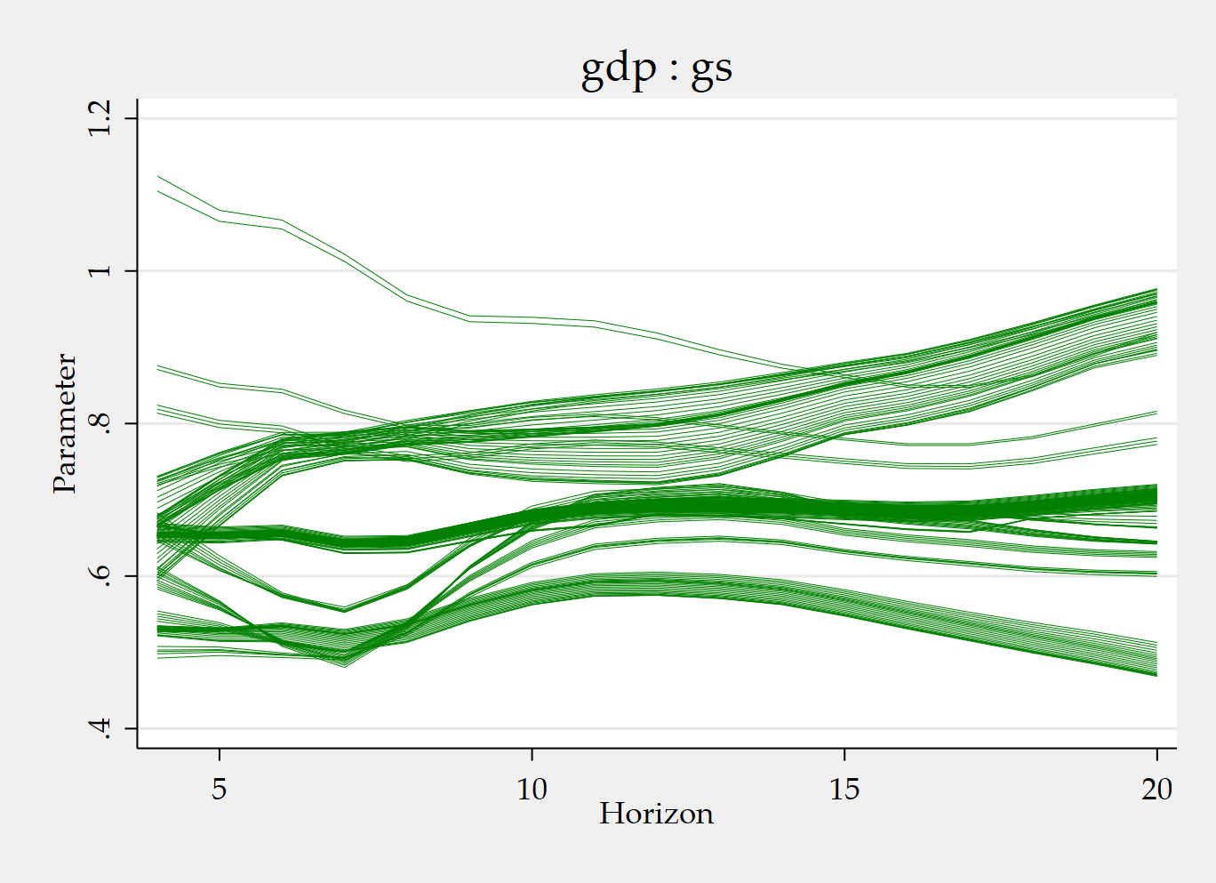
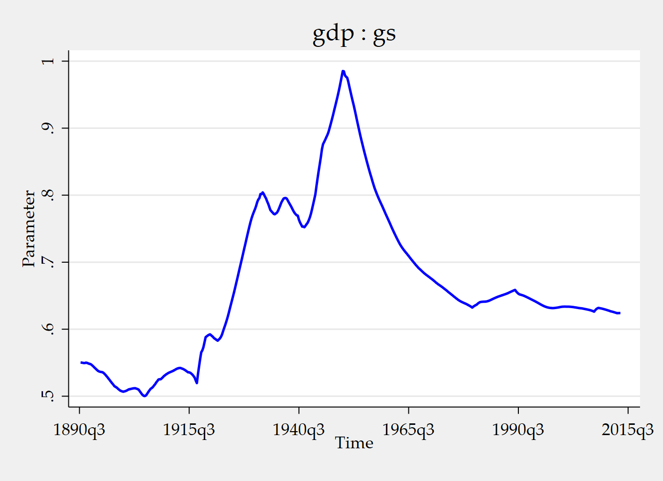
tvpplot, plotcoef(gdp:gs) period(recession) name(figure3_1)
tvpplot, plotcoef(gdp:gs) plotnhor(8) name(figure3_2) Running the code snippet above produce the value of the instrumented cumulative fiscal multiplier during recessions and the time-varying cumulative fiscal multiplier after two years (8 quarters). The instrument is a news shock.
It might be useful to give some explanations about the Mata part:
mata: cB = (3*(0::5))'; cB = cB # J(1,6,1)
This creates the instability grid for the slope block of the parameter vector. The expression 0::5 generates the sequence 0, 1, 2, 3, 4, 5. Multiplying by 3 gives 0, 3, 6, 9, 12, 15. The transpose ' turns that into a column vector. Then cB # J(1,6,1) replicates that grid across 6 columns. So this line builds the grid of admissible instability magnitudes for the slope parameters. Intuitively, the estimator will consider candidate coefficient paths associated with different amounts of time variation, ranging here from no instability to relatively pronounced instability.
mata: cv = (3*(0::5))'; cv = J(1,6,1) # cv
This does the same thing for the covariance block of the parameter vector. Again the grid is 0, 3, 6, 9, 12, 15, but now it is replicated in the way needed for the covariance parameters. So cB controls the instability grid for slopes, while cv controls the instability grid for the covariance terms.
mata: cmat = (J(28,1,1) # cB) \ (J(3,1,1) # cv)
This assembles the full C-grid matrix used by tvpreg. The command says: repeat the slope grid cB for 28 parameters, then stack underneath it the covariance grid cv for 3 parameters. The result is a full block-specific grid for all parameters in the model. In this fiscal-multiplier application, the stacked system has 28 slope parameters and 3 covariance parameters, so this line matches the dimensions of the parameter vector exactly.
This TVP-LP-IV estimate has:
gsas the 1 endogenous regressor ;gdpas the 1 dependent variable ;shockas the 1 excluded instrument ;- included instruments
gs_l* gdp_l* shock_l*plus the constant.
In the paper’s example, those included instruments are:
- 4 lags of
gs; - 4 lags of
gdp; - 4 lags of
shock; - 1 constant.
So,
Therefore,
For the strong-instrument TVP-IV setup used in the paper, the number of slope parameters is
Plugging the numbers in:
Now for the covariance block.
The stacked system has dimension:
so the covariance matrix is 2×2. A symmetric 2×2 matrix has:
mata: st_matrix("cmat",cmat)
This transfers the Mata object cmat into Stata as a standard matrix named cmat, so that the tvpreg command can use it.
This perspective makes it easier to understand the role of cB and cv. In many applications, the full parameter vector contains different blocks, typically a block of slope parameters and a block of covariance parameters. There is no reason to assume that both blocks should be allowed to vary in exactly the same way. The purpose of cB is to define the instability grid for the slope block. The purpose of cv is to define the instability grid for the covariance block. If you use the same values for both, you are allowing roughly the same degree of instability in slopes and covariance terms. If you make cB wider than cv, you are saying that slope coefficients may vary more over time than covariance parameters. So cB and cv are simply block-specific ways of defining the C grid.
That is why changing cB and cv matters. If you choose a narrower grid, such as 0, 2, 4, 6, 8,10, you are restricting the estimator to consider relatively mild instability. If you pick a wider grid, such as 0, 4, 8, 12, 16, 20, you are allowing stronger movement in the coefficient path. So changing cB and cv is not like selecting a different smoothing bandwidth. It is changing the menu of instability magnitudes over which the candidate paths are built and averaged.
The practical takeaway is simple. tvpreg estimates one coefficient path over the full sample for each horizon. It does not obtain time variation by repeatedly re-estimating local regressions. The C grid governs how flexible that full-sample path is allowed to be. Each value in the grid generates a candidate path. The final estimate is then the weighted average of those candidate paths. So when you choose cB and cv, you are deciding which instability scenarios the estimator is allowed to consider for the slope and covariance blocks. That is the key to understanding how tvpreg works and why the C grid is central to the approach.
References
Inoue, A., Rossi, B., & Wang, Y. (2024). Local projections in unstable environments. Journal of Econometrics, 244(2), 105726.
Inoue, A., Rossi, B., Wang, Y., & Zhou, L. (2025). Parameter path estimation in unstable environments: The tvpreg command. The Stata Journal, 25(2), 374-406.
Ginn, W., Saadaoui, J., & Salachas, E. (2025). Stock Price Bubbles, Inflation and Monetary Surprises. Inflation and Monetary Surprises (September 21, 2025).
Müller, U. K., & Petalas, P. E. (2010). Efficient estimation of the parameter path in unstable time series models. The Review of Economic Studies, 77(4), 1508-1539.