During the 24th INFER annual conference, I have the chance to attend the presentation of a very interesting database on bilateral exports by Prof. Dr. Jennifer Pédussel Wu. Crafted in the Aletheia Research Institution, this database aggregates various sources and is available here: https://aletheia-research.org/database-projects/blocs-database/.
Key takeaways
- The Aletheia Research Institution bilateral export database provides valuable trade flow data, which is valuable in the examination of the dynamics of bilateral trade.
- Stata’s areg command greatly enhances the computational efficiency of regression models by estimating several high-dimensional fixed effects and allows for speed gains over other conventional methods.
- The impact of Regional Trade Agreements (RTAs) on bilateral trade is positive but reduces after adjustment for dyadic and time-varying fixed effects, representing the realization of country-specific shocks.
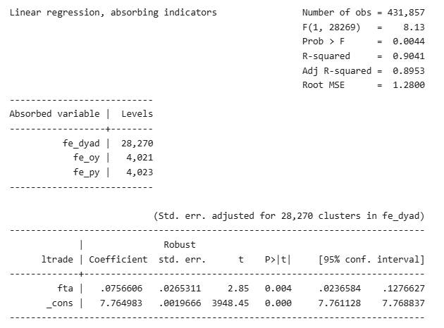
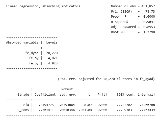
- Free Trade Agreements (FTAs) and Economic Integration Agreements (EIAs) both have a positive impact on trade, with the impact of FTAs being very strong and the impact of EIAs stronger than that of RTAs.
- Applying the use of dyad, exporter-year, and importer-year fixed effects improves the estimates as they minimize bilateral heterogeneity and eliminate trade-related biases.
In this blog, I will show how to use this database to test the areg Stata command that deals with high-dimensional fixed effects (HDFE). As explained on the Stata website, this new command: “absorbs not just one but multiple high-dimensional categorical variables in your linear, fixed-effects linear, and instrumental-variables linear models using option absorb() with commands areg, xtreg, fe, and ivregress 2sls. This provides remarkable speed gains over the traditional approach of directly including indicators for categories of these variables in your models. Choose among different estimation methods.”
How does it work? First, I have to create fixed effects using some Stata syntax and the egen command:

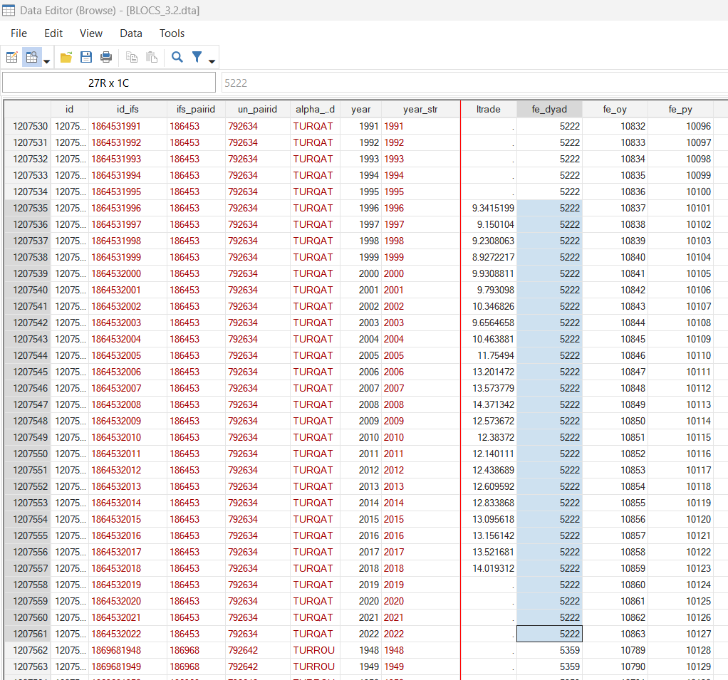
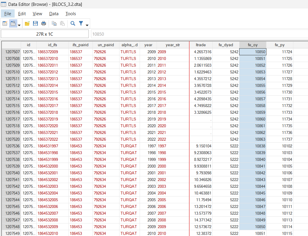
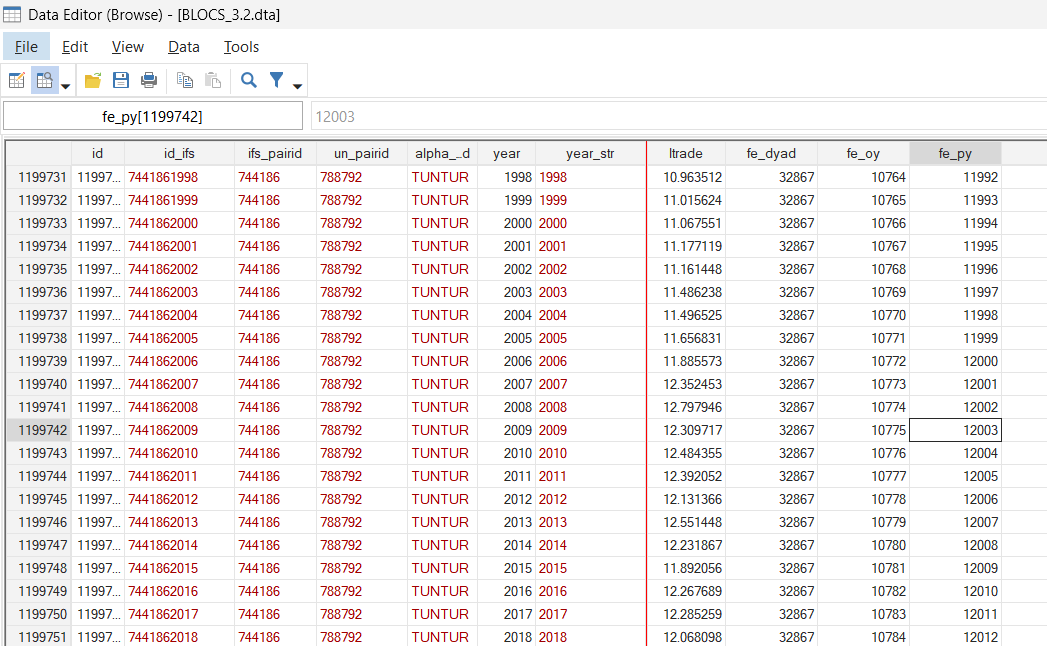
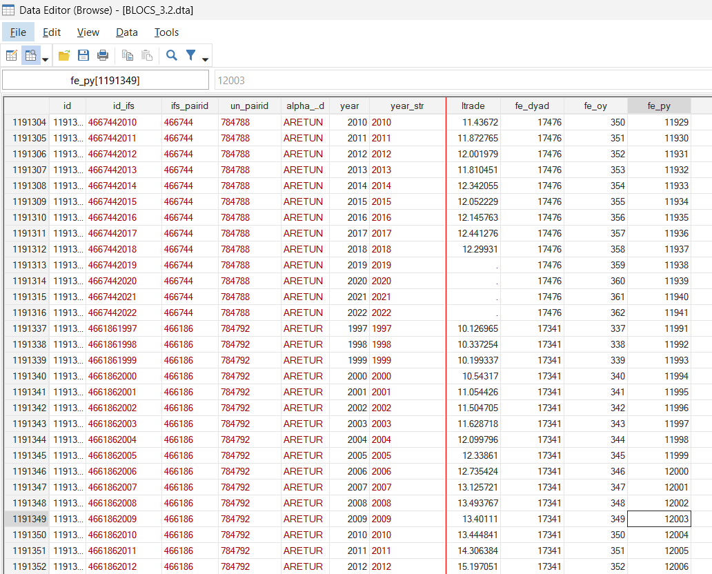
We have created dyadic fixed effects between an exporter and an importer, fixed effects for exporter-year unique combinations, fixed effects for importer year unique combinations.
For example, the dyad Türkiye-Qatar will have the unique number 5222, and the dyad Türkiye-Romania will have the unique number 5359.
The exporter-year fixed effects will produce a unique number, for example, for the combination between Türkiye (as an exporter) and 2009, 10850 in this case.
The importer-year fixed effects will produce a unique number, for example, for the combination between Türkiye (as an importer) and 2009, 12003 in this case.
Now, we can run some regressions and see the effects of including multiple fixed effects:
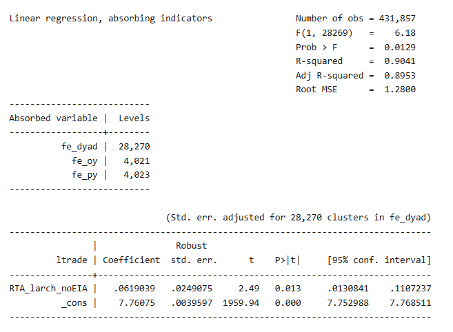
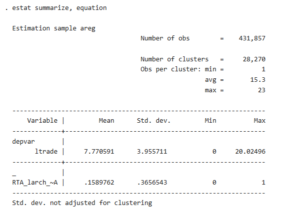
If you only capture dyad fixed effects, the one on RTA_larch_noEIA is big (≈ 0.47) and significant at a very high level, showing that regional trade agreements are positively correlated with increased bilateral trade. When you add some more time-varying fixed effects, the estimates get smaller and in some specifications lose their significance. With origin-year fixed effects, the effect ceases to be significantly different from zero. With fixed effects in partner-year, the coefficient is still positive (≈ 0.10) and significant at the 1% level. Last, with both origin-year and partner-year fixed effects, the coefficient is then robust at around 0.06, significant at the 5% level.
Overall finding is that the trade-increasing impact of RTAs is extremely favorable but significantly diminished once strict fixed effects are controlled for. Implications are that the huge impact in most reduced-form specifications is to some degree motivated by uncontrolled-for time-varying bilateral heterogeneity. After dyad, exporter-year, and importer-year controls are controlled for, RTA effect remains but of mid-size order, meaning RTAs are responsible for trade growth after country-specific shocks and world trends.
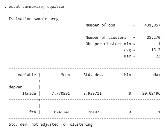
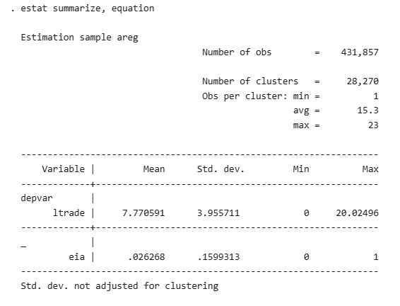
Two additional regressions with Free Trade Agreements and Economic Integration Agreements.
Conclusion
Lastly, this blog shows the strength of the bilateral export dataset of the Aletheia Research Institution with the areg command in Stata to analyze the effect of different trade agreements on bilateral trade. The empirical results indicate that RTAs highly increase trade, but the effect disappears when high-dimensional fixed effects are controlled for, which suggests the contribution of country-specific shocks and global trends to the explanation of growth in trade. This methodology is not only beneficial in research of RTAs but beneficial as well in assessing the FTAs and EIAs impacts. With these tools, researchers can reveal more precise information about patterns of trade that are resistant to contamination due to uncontrolled heterogeneity.
References
Egger, P., & Larch, M. (2008). Interdependent preferential trade agreement memberships: An empirical analysis. Journal of International Economics, 76(2), 384-399.
Wu, J. P., Banach, C. N., Goulas, S., Neira, I. S., Betzelt, S., Hein, E., … & Zimmer, R. (2024). Building BLOCS and stepping stones: combined data for international economic and policy analysis. Berlin School of Economics and Law, Institute for International Political Economy Berlin.