One way to convince some students that it is simple to demonstrate the value of the two first moments of a discrete distribution is to use Mathematica and the Wolfram Language. In this example, we will use the Mean and the Variance of the discrete uniform distribution for purposes of illustration. The notebooks are available at the end of the demonstrations.
The aim is to replicate the demonstrations that can be found here :
https://en.wikibooks.org/
The discrete uniform distribution is where the probability of equally spaced possible values is equal. Mathematically, this means that the probability density function is identical for a finite set of evenly spaced points. An example of would be rolling a fair 6-sided die. In this case, there are six, equally like probabilities.
One common normalization is to restrict the possible values to be integers and the spacing between possibilities to be 1. In this setup, the only two parameters of the function are the minimum value (a), the maximum value (b). Let n=b-a+1 be the number of possibilities.
Mean
Let S={a,a+1,…,b-1,b}. The probability mass function is f(x)=(1/n). The mean (notated as E[X]) can then be derived as follows:
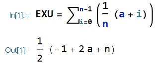
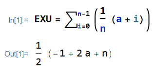
E[X]=\sum_{x \in S} x f(x)\\=\sum_{i=0}^{n-1} \Big(\frac{1}{n}(a+i)\Big)In Wolfram Mathematica, I have:
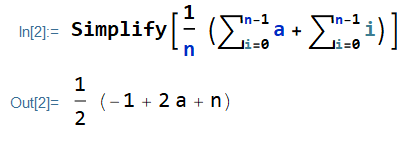
Expand the sum and put aside the term which is not in function of i:
E[X]=\sum_{x \in S} x f(x)\\=\frac{1}{n}\sum_{i=0}^{n-1}a \sum_{i=0}^{n-1}i In Wolfram Mathematica, I have:
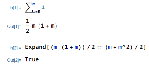
I use the Closed Form for Triangular Numbers, with m (m=n-1):
\begin{align*}
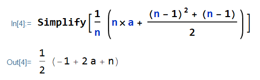
E[X]&=\frac{1}{n}\Big[n\times a \\
&+ \frac{(n-1)^{2}+(n-1)}{2}\Big]
\end{align*}In Mathematica, I have:
\begin{align*}
E[X]&=\Big[(2n\times a \\
&+ n^{2}-2n+1+n-1)/{2n}\Big]
\end{align*}
In Mathematica, I have:
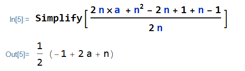
E[X]=\frac{2 a + n-1}{2}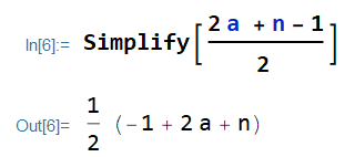
Remember that n=b-a-1.
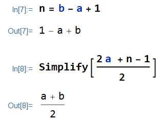
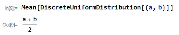
I close the demonstration the mean of the discrete uniform distribution.
Variance
I store the expected value, the mean:
For the variance, I will use the following formula:
V(X) = E[(X-{E}[X])]^{2} \\
{ }\\
= \sum_{x \in S} f(x)(x-E[X])^2 \\
= \sum^{n-1}_{i=0}\Big(\frac{1}{n}\Big((a+i)-{a + b \over 2}\Big)^2\Big)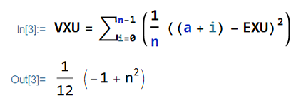
I expand the sum and set aside the term which does not change with i:
V(X) = \frac{1}{n} \sum^{n-1}_{i=0}\Big({a + 2i - b \over 2}\Big)^2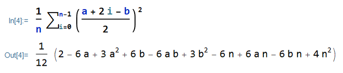
I expand the term in parenthesis:
V(X) = \frac{1}{4n} \sum^{n-1}_{i=0}\Big(a^2 + 4a\times i \\
- 2 a \times  b +4i^{2}-4i\times b + b^2 \Big)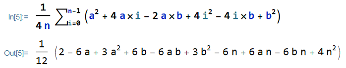
I collect the terms in parenthesis in the sum:
\begin{align*}
V(X) &= \frac{1}{4n} \Big[\sum^{n-1}_{i=0}(a^2 - 2a \times b^2) \\
 &+ \sum^{n-1}_{i=0} (4a\times i -4i\times b) \\
 &+ \sum^{n-1}_{i=0} (4i^2) \Big]
\end{align*}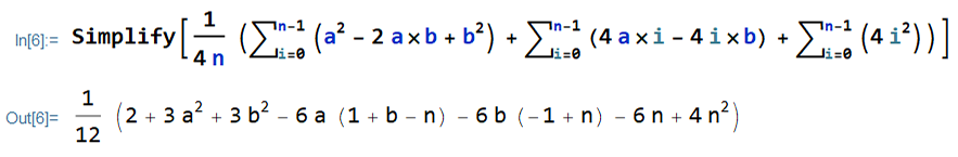
I expand the terms in the three sums:
\begin{align*}
V(X) &= \frac{1}{4n} \Big[n\times(a^2 - 2ab+ b^2) \\
 &+ 4 (a-b) \sum^{n-1}_{i=0} i \\
 &+4 \sum^{n-1}_{i=0} (i^2)  \Big]
\end{align*}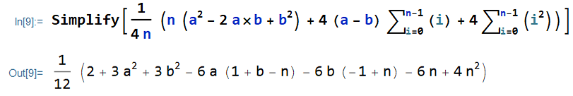
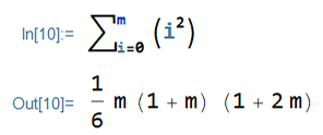
Remember that the sum of the m (m=n-1) squared terms is equal to [m(m+1)(2m+1)]/6:
\begin{align*}
V(X) &= \frac{1}{4n} \Big[n\times(b-a)^2 \\
 &+ 4 (a-b) \bigg( \frac{(n-1)n}{2}\bigg) \\
 &+4 \bigg( \frac{(n-1)n(2n-1)}{6}\bigg)  \Big]
\end{align*}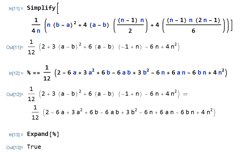
As n=b-a+1 is the number of possibilities, so n-1=b-a:
\begin{align*}
V(X) &= \frac{1}{4n} \Big[n\times(n-1)^2 \\
 &- 2 (n-1) (n-1)n \\
 &+2 (n-1)n(2n-1)/{3}  \Big]
\end{align*}
\begin{align*}
V(X) &= \frac{1}{4} \bigg(-(n-1)^2 \\
&+ {2(n-1)(2n-1) \over 3}  \bigg)
\end{align*}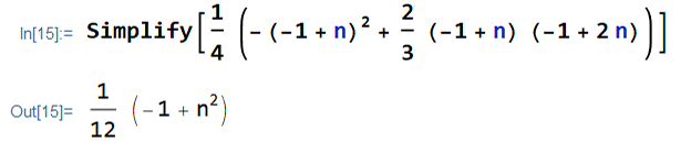
\begin{align*}
V(X) &= \frac{1}{12} \big(-3(n-1)^2 \\
&+ {2(n-1)(2n-1) }  \big)
\end{align*}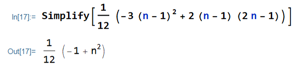
\begin{align*}
V(X) &= \frac{1}{12} \big(-3(n^2-2n+1) \\
&+ 2(2n^2-3n+1)   \big)
\end{align*}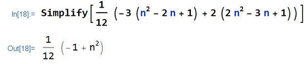
\begin{align*}
V(X) &= \frac{n^2-1}{12}
\end{align*}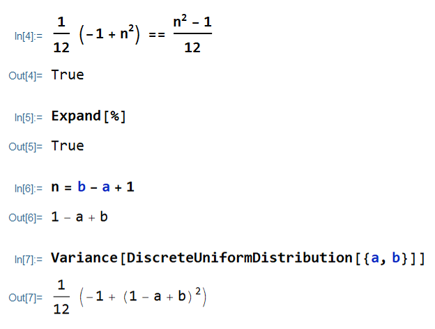
I close the demonstration of the variance.