Logistic growth: clearly explained!

La loi de la population nous est inconnue, parce qu’on ignore la nature de la fonction qui sert de mesure aux obstacles, tant préventifs que destructifs, qui s’opposent à la multiplication indéfinie de l’espèce humaine.

Pierre-François Verhulst (1845).

In this very particular period of Coronacoma for the World Economy, I wrote a brief pedagogical note on the logistic growth. Some observers use this class of model to analyze the new daily infections since they pass through a peak, a maximum before a decline. This kind of analyzes contains many limitations but remains quite interesting.

The title of this note has been inspired by the wonderful YouTuber Josh Starmer of StatQuest.

1. Logistic equation

The logistic equation (sometimes called the Verhulst model or logistic growth curve) is a model of population growth first published by Pierre Verhulst (1845, 1847). The equation [1] is written as follows:

N'[t]=\frac{r N[t] (K-N[t])}{K}

Where r is the Malthusian parameter (rate of maximum population growth) and K is the so-called carrying capacity (i.e., the maximum sustainable population).

Then, divide both sides by K,

\frac{N'[t]}{K}\text{=}\frac{r N[t] \left(1-\frac{N[t]}{K}\right)}{K}

Letting x = N[t] / K, we obtain the following equation [2] :

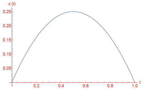
x'(t) = r x(t)(1 - x(t))

Demonstration. From equation 1, we rewrite the corresponding equation is the so-called logistic differential equation:

\dfrac{dN}{dt} = r N \left( 1 - \dfrac{N}{ K} \right)

Analytic Solution. The logistic equation can be solved by separation of variables:

\int \dfrac{ dN } { N \left( 1 - \dfrac{ N }{ K } \right) } = \int r dt 

In order to evaluate the left-hand side, we write:

\begin{aligned}  
\dfrac{ 1 } { N \left( 1 - \dfrac{ N }{ K } \right) } &= \dfrac{ K } { N \left( K - N \right) } \\

\\

 \dfrac{ K } { N \left( K - N \right) } &= \dfrac{1 }{ N} + \dfrac{1 }{ K - N}
\end{aligned}

Hence,

\begin{aligned}

\int \dfrac{ dN }{ N } + \int \dfrac{ dN }{ K - N } &= \int r dt \\

\\

ln| N | - ln| K - N | & = rt + C \\

\\

ln\left|\dfrac{ K - N }{ N }\right| &= -rt - C \\

\\

\left|\dfrac{ K - N }{ N }\right| &= e^{-rt - C} \\

\\

\dfrac{ K - N }{ N } &= Ae^{-rt} \\

\\

(A &= \pm e^{-C})

\end{aligned}

From here we get:

\begin{aligned}

N &= \dfrac{K }{  1 + Ae^{-rt} } \hspace*{1cm} \\

\\

&\left( A = \dfrac{ K - N_0 } { N_0 } = \dfrac{ K} { N_0 } - 1 \right)

\end{aligned}

Note that N₀ is the initial value.

Dividing both sides by K and defining x ≡ N / K. We finally obtain equation [3],

\begin{aligned}

x(t) &= \dfrac{1}{ 1 + Be^{-rt} } \\

\\

& \left( B = \dfrac{ 1} { x_0 } - 1 \right)

\end{aligned}

The function x(t) is sometimes known as the sigmoid function. The following command has been used to plot the continuous version of the logistic model in the Wolfram Language as described in equation 2. The Malthusian parameter is equal to 1 for pedagogical purposes.

Plot[{(1*t*(1 - t))}, {t, 0, 1}]

2. Sigmoid function

The logistic equation has a solution known has the sigmoid function.

The following command has been used to plot the sigmoid function in the Wolfram Language as described in equation 3. The Malthusian parameter is equal to 1 for pedagogical purposes.

Plot[{1/(1 + (1/0.05 - 1)/E^(1*t))}, {t, 0, 10}]

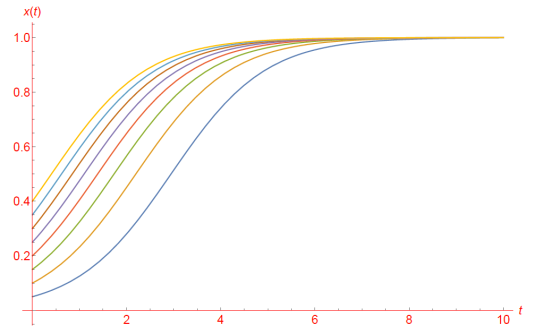
The plot of the solution is shown for initial conditions x₀ = x(t=0) ranging from 0.00 to 0.40 in steps of 0.05.

3. References

• Miguel A. Lerma. Notes on Calculus II. Northwestern University. Accessed 11 April 2020. Retrieved from URL.

• Eric W. Weisstein. Logistic Equation. From MathWorld — A Wolfram Web Resource. Accessed 11 April 2020. Retrieved from URL.