Interactions After Logit: Marginal Effects, Cross-Partials, and Economic Interpretation

Interactions are everywhere in applied economics. We often want to know whether a policy buffer works differently across institutional environments: whether international reserves reduce recession risk more when political stability is high, whether financial development is more stabilizing under weak institutions, or whether trade restrictions weaken the rebound after a global shock.

But when the dependent variable is binary, as in a logit or probit model for the onset of a recession, the interpretation of an interaction term is not as simple as reading the coefficient on $X \times Z$. The key question is, which probability-scale object do we want to interpret?

1. The basic logit model with an interaction

Suppose we estimate a logit model for the onset of a recession:

$$Pr(Recession_i=1)=\Lambda(\eta_i),$$

where$$\eta_i = \alpha + \beta_X X_i + \beta_Z Z_i + \theta X_iZ_i + \gamma’W_i.$$

Here $X_i$​ may be international reserves, financial development, or inflation targeting; $Z_i$​ may be political stability, conflict, or trade restrictions; and $W_i$​ is the vector of controls.

The logit function is:

$$\Lambda(\eta_i)=\frac{\exp(\eta_i)}{1+\exp(\eta_i)}.$$

Let$$p_i=\Lambda(\eta_i).$$

Then:$$\frac{\partial p_i}{\partial \eta_i} = p_i(1-p_i).$$

This is where the nonlinear complication enters. The coefficient $\theta$ is the interaction effect in the latent log-odds index,

$$\frac{\partial^2 \eta_i}{\partial X_i \partial Z_i} = \theta,$$

But it is not the interaction effect on the probability scale.

2. What a standard margins plot computes

When we estimate:

logit recession c.X##c.Z controls, vce(cluster country)
margins, dydx(X) at(Z=(0(.1)1))
marginsplot

Stata computes the marginal effect of $X$ on the probability of recession at different values of $Z$.

For a continuous $X$, the individual marginal effect is:

$$\frac{\partial p_i}{\partial X_i} = p_i(1-p_i)(\beta_X+\theta Z_i).$$

Evaluated at $Z_i=z$, this becomes:

$$ME_{X,i}(z) = p_i(z)[1-p_i(z)](\beta_X+\theta z).$$

The average marginal effect is:

$$AME_X(z) = \frac{1}{N} \sum_{i=1}^{N} p_i(z)[1-p_i(z)](\beta_X+\theta z).$$

This object answers a very natural economic question:

$$\text{What is the effect of } X \text{ on recession risk when } Z \text{ is low, medium, or high?}$$

For example:

$$AME_{IR}(PStab=0),$$$$AME_{IR}(PStab=0.5),$$$$AME_{IR}(PStab=1).$$

This is exactly the kind of object that is useful when the economic question is whether international reserves are more stabilizing in politically stable economies, or whether their buffer role disappears under high trade restrictions.

This approach is not less rigorous than the Ai–Norton approach. It is a different estimand: the level of the marginal effect at meaningful values of the moderator.

Some coding to illustrate the previous point:

*Interactions with one or two
local v "LRESGDP LFI LIT"
local w "LGDeficit LGDebt LCPI LfuelX LfuelM Lfo_r LFM LMIS_CREDIT Lcbie_index LMATR LcurrencyEMP"
local inst "Lconflict_n"
logit RGDP_p `w' (c.(`v')##c.(`inst')), vce(cluster imfcode)
outreg2 using mylogitconf.xls, append ///
dec(3) nonotes
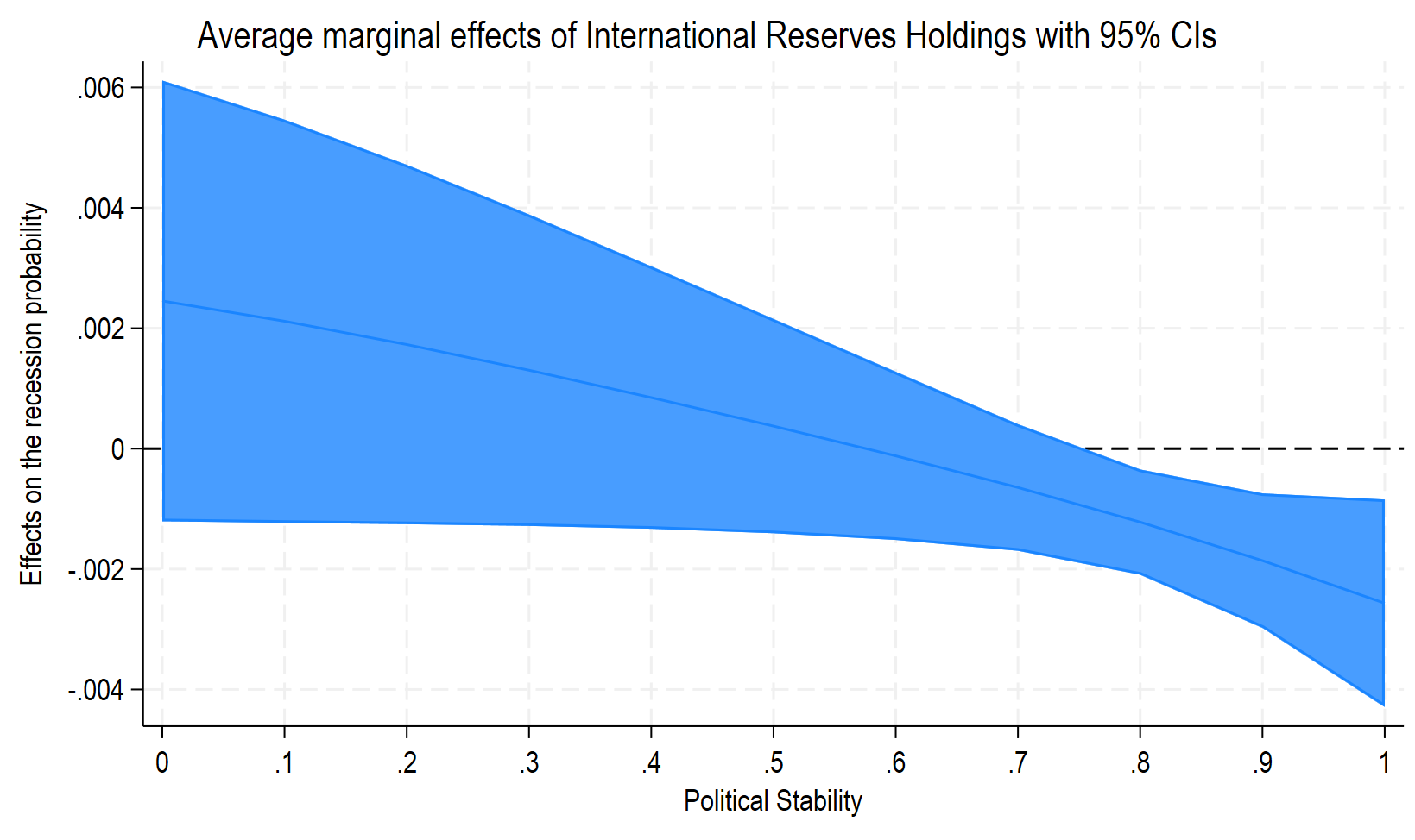
margins, dydx(LRESGDP) at(Lconflict_n=(0(0.1)1)) post

marginsplot, recast(line) recastci(rarea) yline(0) ///
 ti("Average marginal effects of International Reserves Holdings with 95% CIs") ///
 xti("Political Stability") ///
 yti("Effects on the recession probability") name(diffR1, replace)

This gives this very comprehensive figure:

3. What the Ai–Norton object computes

The Ai–Norton object is the cross-partial derivative of the predicted probability:

$$IE_i = \frac{\partial^2 p_i}{\partial X_i \partial Z_i}.$$

For the logit model above, this is:

$$IE_i = p_i(1-p_i) \left[ \theta + (1-2p_i) (\beta_X+\theta Z_i) (\beta_Z+\theta X_i) \right].$$

This object answers a different question:

$$\text{How does the marginal effect of } X \text{ change locally when } Z \text{ changes?}$$

Equivalently,$$IE_i = \frac{\partial}{\partial Z_i} \left( \frac{\partial p_i}{\partial X_i} \right).$$

So the Ai–Norton interaction effect is the slope of the marginal-effect relationship, while the standard margins plot shows the level of the marginal effect.

For probit, the same logic applies. If

$$p_i=\Phi(\eta_i),$$

then the marginal effect of $X$ is:

$$\frac{\partial p_i}{\partial X_i} = \phi(\eta_i)(\beta_X+\theta Z_i),$$

and the cross-partial interaction effect is:

$$IE_i = \phi(\eta_i) \left[ \theta – \eta_i (\beta_X+\theta Z_i) (\beta_Z+\theta X_i) \right].$$

The figure is useful because it shows that the probability-scale interaction effect may vary across observations and across predicted probabilities.

Some coding:

*------------------------------------------------------------*
* 1. Estimate the logit model
*------------------------------------------------------------*

local v "LRESGDP LFI LIT"
local w "LGDeficit LGDebt LCPI LfuelX LfuelM Lfo_r LFM LMIS_CREDIT Lcbie_index LMATR LcurrencyEMP"
local inst "Lconflict_n"

logit RGDP_p `w' c.(`v')##c.(`inst'), vce(cluster imfcode)

outreg2 using mylogitconf.xls, append ///
    dec(3) nonotes

* Optional but useful: check the exact coefficient names
logit, coeflegend

*------------------------------------------------------------*
* 2. Predicted probability, used for the x-axis
*------------------------------------------------------------*

predict double phat_conf if e(sample), pr


*------------------------------------------------------------*
* 3. Correct Ai-Norton interaction effect:
*    d²Pr(RGDP_p=1) / dLRESGDP dLconflict_n
*------------------------------------------------------------*

predictnl double IE_IR_conf = ///
    invlogit(xb())*(1-invlogit(xb())) * ( ///
        _b[c.LRESGDP#c.Lconflict_n] ///
        + (1 - 2*invlogit(xb())) ///
        * (_b[LRESGDP] + _b[c.LRESGDP#c.Lconflict_n]*Lconflict_n) ///
        * (_b[Lconflict_n] ///
            + _b[c.LRESGDP#c.Lconflict_n]*LRESGDP ///
            + _b[c.LFI#c.Lconflict_n]*LFI ///
            + _b[c.LIT#c.Lconflict_n]*LIT) ///
      ) if e(sample), se(SE_IE_IR_conf)


*------------------------------------------------------------*
* 4. z-statistic for the Ai-Norton interaction effect
*------------------------------------------------------------*

gen double Z_IE_IR_conf = IE_IR_conf / SE_IE_IR_conf if e(sample)
gen double P_IE_IR_conf = 2*normal(-abs(Z_IE_IR_conf)) if e(sample)

*------------------------------------------------------------*
* 5. Optional: incorrect logit-style interaction effect
*    This is the common but incomplete calculation:
*    p(1-p)*theta_R
*------------------------------------------------------------*

gen double IE_IR_conf_wrong = ///
    phat_conf*(1-phat_conf)*_b[c.LRESGDP#c.Lconflict_n] if e(sample)


*------------------------------------------------------------*
* 6. Graph 1: correct Ai-Norton interaction effect
*------------------------------------------------------------*

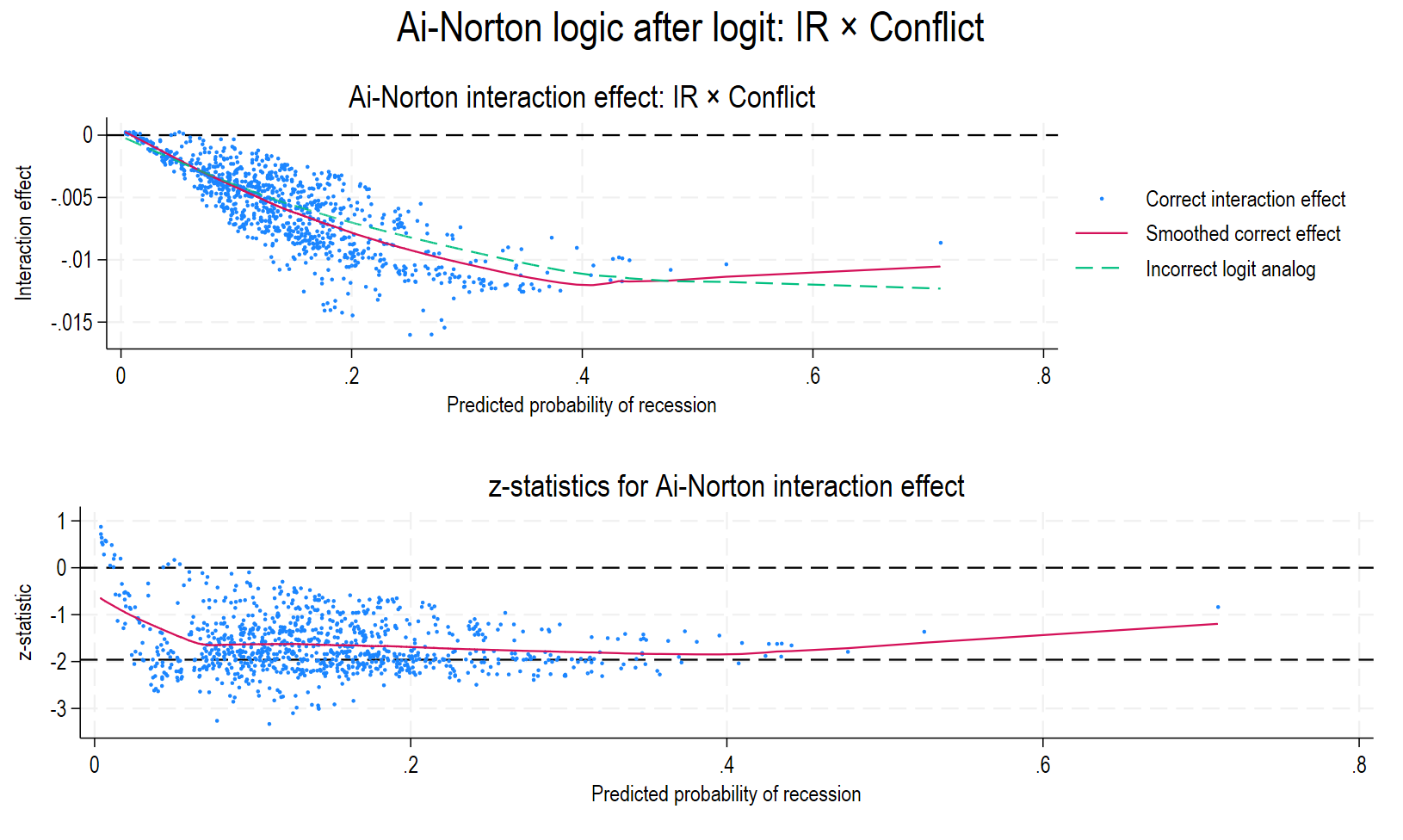
twoway ///
    (scatter IE_IR_conf phat_conf if e(sample), msymbol(oh) msize(tiny)) ///
    (lowess IE_IR_conf phat_conf if e(sample), bwidth(.8)) ///
    (lowess IE_IR_conf_wrong phat_conf if e(sample), bwidth(.8) lpattern(dash)), ///
    yline(0) ///
    xtitle("Predicted probability of recession") ///
    ytitle("Interaction effect") ///
    title("Ai-Norton interaction effect: IR × Conflict") ///
    legend(order(1 "Correct interaction effect" ///
                 2 "Smoothed correct effect" ///
                 3 "Incorrect logit analog")) ///
    name(AN_IE_IR_conf, replace)


*------------------------------------------------------------*
* 7. Graph 2: z-statistics
*------------------------------------------------------------*

twoway ///
    (scatter Z_IE_IR_conf phat_conf if e(sample), msymbol(oh) msize(tiny)) ///
    (lowess Z_IE_IR_conf phat_conf if e(sample), bwidth(.8)), ///
    yline(0 -1.96) ///
    xtitle("Predicted probability of recession") ///
    ytitle("z-statistic") ///
    title("z-statistics for Ai-Norton interaction effect") ///
    legend(off) ///
    name(AN_Z_IR_conf, replace)


*------------------------------------------------------------*
* 8. Combine and export
*------------------------------------------------------------*

graph combine AN_IE_IR_conf AN_Z_IR_conf, col(1) ///
    title("Ai-Norton logic after logit: IR × Conflict")

graph export AiNorton_IR_conflict.png, as(png) replace

This gives the following picture:

4. Why conditional marginal effects are often preferable in macro applications

In macroeconomics, the moderator often has a direct economic interpretation. Political stability ranges from low to high. Trade restrictions range from relatively open to highly restrictive. Political stability may be normalized between 0 and 1.

For this reason, a plot of

$$AME_X(z)$$

against $z$ is often more informative for readers than a plot of

$$\frac{\partial^2 p_i}{\partial X_i \partial Z_i}$$

against the predicted probability.

The first graph says:

At each level of political stability, what is the effect of international reserves on the probability of recession?

The second graph says:

At each predicted probability of recession, what is the local cross-partial interaction effect between international reserves and political stability?

Both questions are meaningful. But the first is usually closer to the policy interpretation.

In our recession-onset application, the substantive statement is not simply that the interaction coefficient is negative. The substantive statement is that the buffer role of macroeconomic variables depends on the institutional or trade environment. In the paper, the logit analysis examines interactions between reserves, financial institutions, inflation targeting, political stability, and trade restrictions. The results are then translated into marginal effects at low, intermediate, and high values of the moderator.

That is the right object for a macro-policy claim such as:

International reserves reduce recession risk only when political stability is sufficiently high.

or:

The stabilizing role of reserves weakens when trade restrictions are high.

5. The threshold interpretation

One useful feature of the logit model is that the sign of the marginal effect of a continuous $X$ is governed by the latent-index slope:

$$\beta_X+\theta z.$$

This is because the logit density term is always positive:

$$p_i(z)[1-p_i(z)]>0.$$

Therefore,

$$\text{sign}\left(ME_{X,i}(z)\right) = \text{sign}(\beta_X+\theta z).$$

The threshold value of $Z$Z at which the marginal effect changes sign is:

$$z^* = -\frac{\beta_X}{\theta}.$$

This threshold is meaningful if it is computed from the underlying logit coefficients. It should not be computed by mechanically combining already-reported marginal effects.

The probability-scale magnitude is still:

$$p_i(z)[1-p_i(z)](\beta_X+\theta z),$$

but the sign switch occurs when:

$$\beta_X+\theta z=0.$$

This explains why threshold statements can be useful in macro papers. They summarize the institutional or trade environment under which a macroeconomic buffer starts to reduce recession risk.

6. What is actually incorrect?

The conditional marginal-effects approach is not incorrect. The Ai–Norton cross-partial approach is not superior. The mistakes are elsewhere.

First, it is incorrect to interpret $\theta$, the coefficient on $X \times Z$, as the interaction effect on the probability scale.

Second, it is incorrect to say that the probability-scale marginal effect is simply:

$$\beta_X+\theta z.$$

That is the effect on the latent logit index, not on the probability. The probability-scale effect is:

$$p_i(z)[1-p_i(z)](\beta_X+\theta z).$$

Third, it is generally incorrect to take reported marginal effects from a table and compute:

$$ME_X+zME_{XZ}.$$

That does not reproduce the correct logit marginal effect, because the nonlinear scaling term

$$p_i(z)[1-p_i(z)]$$

changes with $z$, with $X_i$​, and with the other covariates.

The correct approach is to compute the marginal effects directly from the estimated nonlinear model, using the full variance-covariance matrix.

7. Stata implementation

For the conditional marginal-effect approach, the code should use factor-variable notation:

logit RGDP_p ///
    LGDeficit LGDebt LCPI LfuelX LfuelM Lfo_r LFM ///
    LMIS_CREDIT Lcbie_index LMATR LcurrencyEMP ///
    c.LRESGDP##c.Lconflict_n ///
    c.LFI##c.Lconflict_n ///
    i.LIT##c.Lconflict_n, ///
    vce(cluster imfcode)margins, dydx(LRESGDP) ///
     at(Lconflict_n=(0(.1)1))marginsplot, recast(line) ///
     recastci(rarea) yline(0) ///
    title("Average marginal effects of international reserves") ///
    xtitle("Conflict") ///
    ytitle("Effect on the probability of a recession")

The factor-variable notation is important. It tells Stata that the interaction term changes when the underlying variable changes. This is essential for correct marginal effects.

For an Ai–Norton-style cross-partial after logit, the object is:

$$\frac{\partial^2 Pr(Recession_i=1)} {\partial LRESGDP_i \partial Lconflict\_n_i}.$$

If the estimated model includes interactions between conflict and several variables,

$$\eta_i = \gamma’W_i + \beta_R R_i + \beta_F F_i + \beta_T T_i + \delta C_i + \theta_R R_iC_i + \theta_F F_iC_i + \theta_T T_iC_i,$$

then the cross-partial for $R_i=LRESGDP_i$​ and $C_i=PStab\_n_i$​ is:

$$IE_i = p_i(1-p_i) \left[ \theta_R + (1-2p_i) (\beta_R+\theta_R C_i) (\delta+\theta_R R_i+\theta_F F_i+\theta_T T_i) \right].$$

In Stata, this can be computed with predictnl:

predict double phat_conf if e(sample), prlocal p "invlogit(xb())"local deta_dR ///
    "_b[LRESGDP] + _b[c.LRESGDP#c.Lconflict_n]*Lconflict_n"local deta_dC ///
    "_b[Lconflict_n] ///
    + _b[c.LRESGDP#c.Lconflict_n]*LRESGDP ///
    + _b[c.LFI#c.Lconflict_n]*LFI ///
    + _b[1.LIT#c.Lconflict_n]*LIT"predictnl double IE_IR_conf = ///
    (`p')*(1-(`p')) * ( ///
        _b[c.LRESGDP#c.Lconflict_n] ///
        + (1 - 2*(`p')) * (`deta_dR') * (`deta_dC') ///
    ) if e(sample), se(SE_IE_IR_conf)gen double Z_IE_IR_conf = IE_IR_conf / SE_IE_IR_conf if e(sample)

This gives the observation-level cross-partial interaction effect and its $z$z-statistic. A figure can then plot IE_IR_conf and Z_IE_IR_conf against phat_conf, following the Ai–Norton visual logic.

8. A useful way to describe both figures

The conditional marginal-effect figure can be described as:

The figure reports the average marginal effect of international reserves on the probability of entering a recession, evaluated at different levels of conflict. The estimates are computed from the logit model, with standard errors obtained using the delta method.

The Ai–Norton-style figure can be described as:

The figure reports the nonlinear cross-partial interaction effect between international reserves and conflict after logit, $\partial^2 Pr(Recession=1)/\partial LRESGDP \partial Lconflict\_n$∂2, evaluated for each observation and plotted against the predicted probability of recession.

Neither figure is more rigorous. They answer different questions.

The first asks:

$$\text{How large is the effect of } X \text{ at each level of } Z?$$

The second asks:

$$\text{How does the effect of } X \text{ change locally as } Z \text{ changes?}$$

---

9. The bottom line

For macroeconomic interpretation, I would usually keep conditional average marginal effects as the main presentation. They are transparent, policy-relevant, and directly tied to the economic mechanism.

The Ai–Norton cross-partial is useful as an additional representation of the nonlinear interaction structure. It shows whether the local interaction effect on the probability scale is positive or negative across the distribution of predicted probabilities.

The cleanest methodological statement is therefore:

In the main analysis, we report conditional average marginal effects: the effect of a macroeconomic variable on the probability of recession evaluated at selected levels of the institutional or trade-policy moderator. As a complementary exercise, we compute the nonlinear cross-partial interaction effect in the spirit of Ai and Norton. These two objects are not substitutes; they answer different but related questions.

In short, after logit or probit, do not interpret the interaction coefficient mechanically. Work on the probability scale. But once on the probability scale, choose the estimand that corresponds to the economic question. For macro-policy interpretation, the conditional marginal effect is often the clearest object.

Reference

Ai, C., & Norton, E. C. (2003). Interaction terms in logit and probit models. Economics Letters, 80(1), 123–129.

Aizenman, J., Ito, H., Park, D., Saadaoui, J., & Uddin, G. S. (2025). Global shocks, institutional development, and trade restrictions: What can we learn from crises and recoveries between 1990 and 2022?. Journal of International Money and Finance, 103504.

Norton, E. C., Wang, H., & Ai, C. (2004). Computing interaction effects and standard errors in logit and probit models. The Stata Journal, 4(2), 154–167.

Marigo, J.-B., & Weill, L. (2025). Once upon a loan: How folk tales shape access to credit. Journal of Economic Behavior and Organization, 239, 107288.