In a future work in preparation, we will explore how geopolitical relationship shocks, such as changes in US-China, China-Japan, or China-India relations, affect provincial GDP growth in China. Methodologically, the analysis combines two complementary strands developed in earlier posts:
- Local projections with Driscoll-Kraay inference, suitable for short panels with strong cross-sectional dependence
- Heterogeneous difference-in-differences and AIPW estimators, designed to capture nonlinear and state-dependent effects
This post explains why combining these tools is not only coherent, but informative.
1. Baseline dynamics: Local projections with DK inference
The starting point follows the framework discussed in my previous blog:“Drawing local projection IRFs with Driscoll–Kraay inference in Stata”.
Using local projections (LPs), I estimate horizon-specific responses of provincial GDP growth to common geopolitical shocks, allowing for flexible dynamics and avoiding VAR misspecification. Given the panel structure (around 31 provinces over roughly 20 years), Driscoll–Kraay standard errors are used to account for:
- cross-sectional dependence,
- serial correlation,
- and heteroskedasticity.
These LP–DK impulse responses provide a linear, average marginal effect of a one-standard-deviation change in political relations. For example, improvements in US–China relations are associated with positive short-run responses in provincial growth, while the medium-run effects tend to attenuate.
This baseline is conservative by construction and well suited as a reference specification.
2. Why linear IRFs are not enough
However, geopolitical shocks are rarely “small.” Large deteriorations or large improvements may trigger qualitatively different adjustment mechanisms:
- policy responses,
- reallocation across provinces,
- trade diversion,
- or substitution toward domestic demand.
Linear LPs implicitly assume proportionality. To relax this assumption, I turn to quantile-based treatment definitions.
3. Quantile-based AIPW event studies
Building on the ideas discussed in in my previous blog: “Heterogeneous difference-in-differences with Stata”, I implement a quantile-based AIPW event-study design.
The logic is simple:
- Large improvements in political relations are defined as shocks in the top quartile of the standardized distribution.
- Large deteriorations correspond to the bottom quartile.
- The middle 50% of observations serves as the control group.
For each horizon h=0,1,2, I estimate average treatment effects (ATEs) using the augmented inverse probability weighting (AIPW) estimator, which is doubly robust to misspecification of either the outcome or treatment model.
This delivers IRF-style ATEs that are explicitly nonlinear and state-dependent.
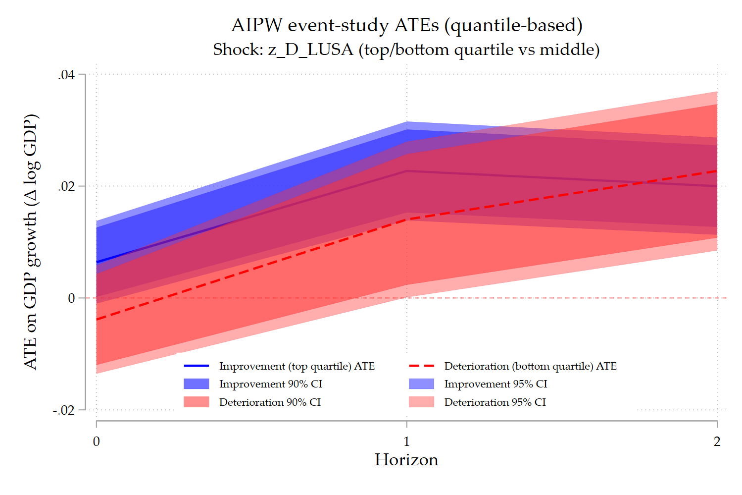
4. Interpreting the results
Three key findings emerge:
- Large improvements in political relations have consistently positive effects on provincial GDP growth, peaking around one year after the shock.
- Large deteriorations also display positive medium-run ATEs relative to moderate shocks.
- This does not contradict the linear LP results: the benchmark here is the middle of the shock distribution, not a zero-shock counterfactual.
In other words, severe deteriorations appear to activate compensating mechanisms (policy support, reallocation, or substitution) that mitigate or even reverse short-run losses relative to milder shocks.
5. Why the two approaches are complementary
The contribution of this framework lies in the joint use of:
- LPs with DK inference → credible, conservative average dynamics under cross-sectional dependence;
- Quantile-based AIPW event studies → nonlinear, distribution-aware causal effects.
Together, they provide a richer picture of how geopolitical shocks propagate through a large, heterogeneous economy like China’s.
6. Takeaway
Linear IRFs answer the question:
What is the average marginal effect of a small change in geopolitical relations?
Quantile-based AIPW answers a different one:
What happens when relations improve or deteriorate sharply, compared to “normal” times?
Using both is not redundant, it is necessary.
Full code for pedagogical purposes:
*============================================================
* AIPW event-study ATEs (quantile-based) with visible CIs
* - Common shock: `shock' (e.g., z_D_LUSA)
* - Treatment: top quartile (improvement) vs middle; bottom quartile (deterioration) vs middle
* - Horizon outcomes: y_h = F^h D.GDP, h=0..H
* - AIPW with vce(cluster unit_id)
* - Plots ATEs with 90% and 95% CIs (dark enough to see)
*
* REQUIREMENTS:
*   xtset unit_id period
*   shock variable exists (e.g., z_D_LUSA)
*   D.GDP exists
*============================================================

preserve

*----------------------------
* 0) Panel setup
*----------------------------
xtset unit_id period

cls

* Shock (change if needed)
local shock "z_D_LUSA"

* Horizon
local H 2

*----------------------------
* 1) Pre-generate lags (teffects does NOT allow L. operators)
*----------------------------
foreach v in CPI TRADE GFCF POP TOT {
    capture drop L1_`v' L2_`v'
    gen double L1_`v' = L1.`v'
    gen double L2_`v' = L2.`v'
}

capture drop L1_DGDP L2_DGDP
gen double L1_DGDP = L1.D.GDP
gen double L2_DGDP = L2.D.GDP

local X "L1_CPI L2_CPI L1_TRADE L2_TRADE L1_GFCF L2_GFCF L1_POP L2_POP L1_TOT L2_TOT L1_DGDP L2_DGDP"

*----------------------------
* 2) Create horizon outcomes y_h = F^h D.GDP
*----------------------------
forvalues h = 0/`H' {
    capture drop y`h'
    gen double y`h' = F`h'.D.GDP
}

*----------------------------
* 3) Define quantile-based events (computed over available shock observations)
*----------------------------
quietly summarize `shock' if !missing(`shock'), detail
local q25 = r(p25)
local q75 = r(p75)

capture drop imp det mid check
gen byte imp = (`shock' >= `q75') if !missing(`shock')
gen byte det = (`shock' <= `q25') if !missing(`shock')
gen byte mid = (`shock' >  `q25' & `shock' < `q75') if !missing(`shock')

* Sanity checks
tab imp
tab det
tab mid
gen byte check = imp + det + mid
tab check if !missing(`shock')   // should be 1

summ z_D_LUSA if det==1
summ z_D_LUSA if imp==1

*----------------------------
* 4) AIPW by horizon: improvements vs middle AND deteriorations vs middle
*----------------------------
tempfile res_imp res_det
tempname post_imp post_det

postfile `post_imp' int h double ate se lo95 hi95 lo90 hi90 using `res_imp', replace
postfile `post_det' int h double ate se lo95 hi95 lo90 hi90 using `res_det', replace

forvalues h = 0/`H' {

    * z critical values (teffects uses asymptotic normal inference)
    scalar z95 = invnormal(0.975)
    scalar z90 = invnormal(0.95)

    *----------------------------
    * Improvements: imp==1 vs mid==1
    *----------------------------
    quietly teffects aipw (y`h' `X') (imp `X') if imp==1 | mid==1, vce(cluster unit_id)

    matrix b = e(b)
    matrix V = e(V)
    scalar ate = b[1,1]
    scalar se  = sqrt(V[1,1])

    scalar lo95 = ate - z95*se
    scalar hi95 = ate + z95*se
    scalar lo90 = ate - z90*se
    scalar hi90 = ate + z90*se

    post `post_imp' (`h') (ate) (se) (lo95) (hi95) (lo90) (hi90)

    *----------------------------
    * Deteriorations: det==1 vs mid==1
    *----------------------------
    quietly teffects aipw (y`h' `X') (det `X') if det==1 | mid==1, vce(cluster unit_id)

    matrix b = e(b)
    matrix V = e(V)
    scalar ate = b[1,1]
    scalar se  = sqrt(V[1,1])

    scalar lo95 = ate - z95*se
    scalar hi95 = ate + z95*se
    scalar lo90 = ate - z90*se
    scalar hi90 = ate + z90*se

    post `post_det' (`h') (ate) (se) (lo95) (hi95) (lo90) (hi90)
}

postclose `post_imp'
postclose `post_det'

*----------------------------
* 5) Merge results and plot (bands visible)
*----------------------------
use `res_imp', clear
rename ate  ate_imp
rename se   se_imp
rename lo95 lo95_imp
rename hi95 hi95_imp
rename lo90 lo90_imp
rename hi90 hi90_imp
tempfile tmp_imp
save `tmp_imp', replace

use `res_det', clear
rename ate  ate_det
rename se   se_det
rename lo95 lo95_det
rename hi95 hi95_det
rename lo90 lo90_det
rename hi90 hi90_det

merge 1:1 h using `tmp_imp', nogen
sort h

* Quick check: make sure CIs exist (optional)
list h ate_imp lo90_imp hi90_imp lo95_imp hi95_imp ate_det lo90_det hi90_det lo95_det hi95_det, noobs

* Plot: darker opacity so CIs show clearly in export
twoway ///
    (rarea hi95_imp lo95_imp h, sort fcolor(blue%55) lcolor(blue) ///
	lwidth(vvthin)) ///
    (rarea hi90_imp lo90_imp h, sort fcolor(blue%70) lcolor(blue) ///
	lwidth(vvthin)) ///
    (line  ate_imp h, sort lcolor(blue) lwidth(medthick)) ///
    (rarea hi95_det lo95_det h, sort fcolor(red%40) lcolor(red) ///
	lwidth(vvthin)) ///
    (rarea hi90_det lo90_det h, sort fcolor(red%55)  lcolor(red) ///
	lwidth(vvthin)) ///
    (line  ate_det h, sort lcolor(red) lwidth(medthick) lpattern(dash)) ///
    , yline(0, lcolor(red%35)) ///
      xlabel(0 1 2) xscale(range(0 `H')) ///
      xtitle("Horizon") ///
      ytitle("ATE on GDP growth (Δ log GDP)") ///
      title("AIPW event-study ATEs (quantile-based)") ///
      subtitle("Shock: `shock' (top/bottom quartile vs middle)") ///
      legend(order(3 "Improvement (top quartile) ATE" ///
                   6 "Deterioration (bottom quartile) ATE" ///
                   2 "Improvement 90% CI" 1 "Improvement 95% CI" ///
                   5 "Deterioration 90% CI" 4 "Deterioration 95% CI") ///
             cols(2) pos(6) ring(0) region(lcolor(none))size(*0.8)) ///
      graphregion(color(white)) plotregion(color(white)) name(aipw`v', replace)

restore
2 Comments
Amazing and valuable contribution.
Thank you! You have to check some paper for the inference in the LP-AIPW estimator.