Introduction
This short note aims to demonstrate the drawing of choropleth maps at different regional levels thanks to geoboundary, the Stata package provided by Asjad Naqvi. Drawing maps on Stata may be perceived as complex by some practitioners and, particularly, by students. In the following, I will show you how to draw the three following maps
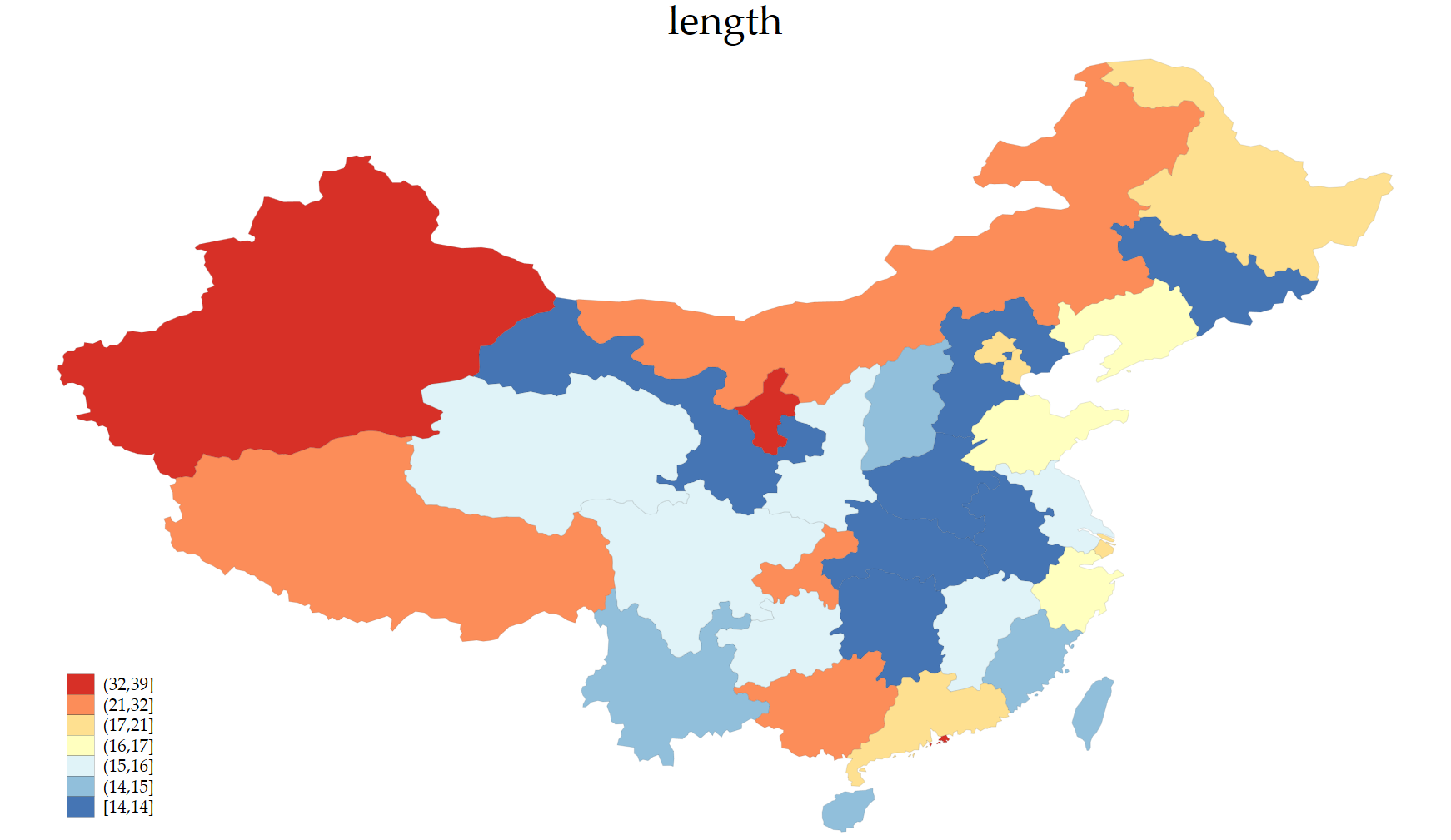
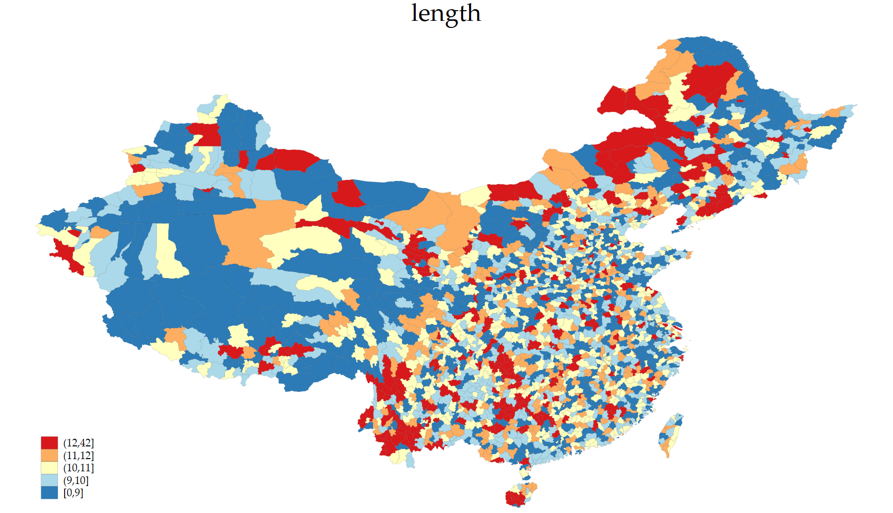

The maps shown above correspond to three levels of aggregation. The first map displays province-level averages. The second map displays prefecture-level averages. The third map displays county-level values. For each map the color scale reflects the length of the administrative name, measured with the length(shapeName) function.
*cd "C:\Users\jamel\Downloads\"

ssc install geoboundary, replace

geoboundary CHN, level(ADM3)

geoboundary CHN, level(ADM3) replace convert

use CHN_ADM3, clear

grmap using CHN_ADM3_shp, id(_ID)

////////////////////////////////////////////////////////////////

**# Some colors

set scheme Cleanplots
graph set window fontface "Palatino Linotype"

generate length = length(shapeName)

grmap length using CHN_ADM3_shp, id(_ID) fcolor(BuYlRd) ///
osize(vvthin .. ) ndsize(vvthin) ndfcolor(gray) ///
title("length") clnumber(7) name(ADM3, replace)

///////////////////////////////////////////////////////////////

geoboundary CHN, level(ADM2)

geoboundary CHN, level(ADM2) replace convert

use CHN_ADM2, clear

grmap using CHN_ADM2_shp, id(_ID)

////////////////////////////////////////////////////////////////

**# Some colors

set scheme Cleanplots
graph set window fontface "Palatino Linotype"

generate length = length(shapeName)

grmap length using CHN_ADM2_shp, id(_ID) fcolor(BuYlRd) ///
osize(vvthin .. ) ndsize(vvthin) ndfcolor(gray) ///
title("length") clnumber(7) name(ADM2, replace)

///////////////////////////////////////////////////////////////

geoboundary CHN, level(ADM1)

geoboundary CHN, level(ADM1) replace convert

use CHN_ADM1, clear

grmap using CHN_ADM1_shp, id(_ID)

////////////////////////////////////////////////////////////////

**# Some colors

set scheme Cleanplots
graph set window fontface "Palatino Linotype"

generate length = length(shapeName)

grmap length using CHN_ADM1_shp, id(_ID) fcolor(BuYlRd) ///
osize(vvthin .. ) ndsize(vvthin) ndfcolor(gray) ///
title("length") clnumber(7) name(ADM1, replace)

////////////////////////////////////////////////////////////////
What the province map reveals
The province map displays very clear spatial clustering. Western provinces such as Xinjiang and Tibet show the longest names. Coastal provinces such as Zhejiang, Fujian, and Guangdong show shorter averages. This pattern reflects linguistic and historical differences. Regions with strong minority presence or long descriptive toponyms naturally produce longer administrative names. Regions with older and more standardized naming traditions display more concise labels.
What the prefecture map adds
Moving to the prefecture map increases the level of detail and immediately reveals large within-province differences. Several interior provinces display prefectures with long names adjacent to prefectures with much shorter names. This richer variation suggests that toponymic structure is not only driven by broad regional identity but also by historical decisions made at subnational levels, sometimes inherited from older administrative systems.
What the county map shows
The county-level map is the most detailed and the most striking. At this resolution China appears as a mosaic. Clusters of long names and clusters of short names appear even within the same prefecture. The highest values are observed in parts of the southwest and along certain historical frontier regions. The provincial capitals and major prefectures appear as small pockets with short names, consistent with urban administrative simplification.
The three maps together illustrate the importance of administrative resolution in any spatial analysis. A pattern that appears smooth at the province level becomes far more complex at the county level. For applied research in economic geography, development studies, political economy, or environmental shocks, the choice of administrative scale can fundamentally change the interpretation of spatial patterns.
Final remark
This example uses a trivial variable but demonstrates a powerful idea. Stata can produce high-quality maps with clean design, well-calibrated color schemes, and transparent reproducibility. The geoboundary package simplifies access to global administrative boundaries, and grmap provides a flexible platform for turning those boundaries into informative graphics.