Before reading this blog, I recommend you to read the first 5 parts of this blog series. Available below:
Do geopolitical risks raise or lower inflation? Part VI
Spillovers: can foreign geopolitical risk raise domestic inflation?
In the previous posts, I focused on a sequence of increasingly demanding questions. First, does higher geopolitical risk raise inflation in the long historical panel? Then, do acts differ from threats? Do global shocks differ from country-specific shocks? Does the result survive a narrative identification check? And, finally, does the basic inflationary pattern remain once one moves away from the pooled estimator and allows for cross-country heterogeneity? The answer to all of these questions was broadly reassuring. The inflationary effect survives.
This final post turns to what is, in many ways, the most international question in the paper by Dario Caldara, Sarah Conlisk, Matteo Iacoviello, and Maddie Penn: what happens when geopolitical risk rises abroad rather than at home? This is the purpose of Figure 9. Instead of asking how a domestic geopolitical shock affects domestic inflation and activity, the figure asks whether foreign geopolitical tensions spill over into the domestic economy. That is a crucial question in a world where trade, commodity prices, financial markets, and expectations are tightly interconnected. The paper’s broader motivation is precisely that geopolitical tensions can move inflation through supply, demand, and policy channels, and not only through direct domestic conflict.
The empirical setup is elegant. For each country, the authors estimate a 4-variable VAR including domestic GPR, foreign GPR, inflation, and real GDP. A geopolitical spillover shock is defined as an exogenous increase in the GPR of other countries while holding domestic GPR constant on impact. The figure then compares 3 estimators: the pooled baseline, the inverse-variance-weighted average of country-by-country VARs, and the equally weighted average. In other words, Figure 9 combines the logic of international spillovers with the logic of heterogeneity already explored in Figure 7.
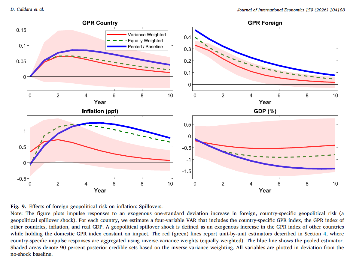
The first thing I like about this figure is that it sharpens the interpretation of geopolitical risk as a genuinely international macroeconomic disturbance. A country does not need to be the epicenter of the geopolitical event to feel its consequences. If tensions rise elsewhere, domestic inflation can still increase and domestic GDP can still decline. That is precisely what one would expect if the main transmission mechanisms run through cross-border channels such as commodity prices, trade, confidence, and international financial conditions. The figure therefore extends the argument of the earlier posts: geopolitical risk is not only a domestic shock; it is also an imported shock.
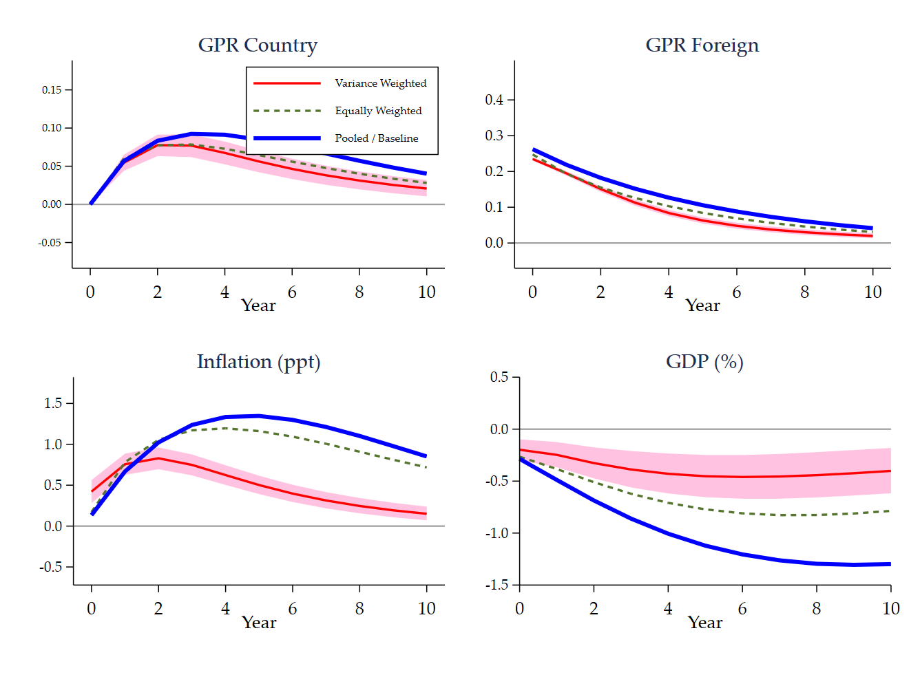
The replication is especially instructive because it forced an important technical clarification. Figure 7 and Figure 9 may look visually similar, but they are not the same econometric object. Figure 7 is a normalized comparison across estimators. Figure 9 is not. For the spillover exercise, the impulse responses have to remain in original units. Once that distinction is respected, the figure falls into place. The foreign GPR response starts positive and then decays gradually. Domestic GPR rises only modestly after the foreign shock, which is accurately what one would expect from a spillover mechanism rather than a direct domestic disturbance. Inflation rises, and GDP falls. In qualitative terms, that is the right picture. It is also the right economic interpretation. The spillover shock looks stagflationary.
Substantively, the most interesting comparison is between the pooled and unit-by-unit estimators. In the inflation panel, the pooled response is stronger and more persistent than the inverse-variance-weighted response, while the equally weighted estimator sits much closer to the pooled path. That pattern is informative. It suggests that the average spillover effect is real, but also that countries differ substantially in the intensity with which foreign geopolitical tensions feed into domestic inflation. The weighted estimator gives more influence to countries whose responses are estimated more precisely, and those countries appear to display a more moderate inflation response than the pooled system. This is not a contradiction. It is undoubtedly what one should expect in the presence of heterogeneous international exposure.
The GDP panel is, in my view, even more revealing. The pooled estimator shows a much larger and more persistent contraction than the 2 unit-by-unit aggregates. So the conclusion is not simply that foreign geopolitical risk is recessionary. It is that the pooled cross-country system translates the common international component of the shock into a stronger average output loss than what emerges from precision-weighted or equally weighted country-by-country estimation. This is useful because it reminds us that pooled systems and mean-group systems are answering slightly different questions. The pooled estimator captures a common dynamic structure. The unit-by-unit estimators summarize a distribution of country-specific dynamics. Both are informative, but they need not coincide exactly. That was already the lesson of Part V, and Figure 9 shows that the lesson becomes even more important once spillovers are involved.
What does all this tell us economically? It tells us that geopolitical fragmentation can transmit across borders even when countries are not themselves experiencing the original adverse event. A rise in foreign geopolitical risk may weaken activity through external demand, trade disruptions, commodity-price pressures, or broader uncertainty, while at the same time pushing inflation upward. That is a very uncomfortable configuration for policymakers. It means that the inflationary consequences of geopolitical turmoil cannot be analyzed only through domestic event studies. International exposure matters. Spillovers matter. And, in a connected world economy, they matter a lot.
More broadly, Figure 9 is a fitting way to end this blog series. By the time one reaches this point, the paper’s central result has survived a wide range of challenges. The baseline pooled historical VAR says geopolitical risk is inflationary and contractionary. The acts-threats decomposition preserves that conclusion. The global-country decomposition preserves it. The narrative identification check preserves it. The mean-group comparison preserves it. And now the spillover exercise shows that even foreign geopolitical risk can generate the same broad configuration. By this stage, the message is challenging to dismiss: geopolitical risk is not a narrow or local disturbance. It is a macroeconomic force with broad historical reach, heterogeneous national consequences, and strong cross-border transmission.
From a replication perspective, this last figure is also a nice reminder of what successful replication really means. It is not only about drawing a similar line. It is about understanding the economic object one is trying to reproduce. In this case, the key step was to recognize that the spillover IRFs should remain unnormalized. Once that was done, the Stata/Mata replication became coherent both visually and economically. For me, that is the main pedagogical value of the whole exercise. Replication is not mechanical copying. It is a way to understand why a figure looks the way it does, what assumptions sit behind it, and what economic interpretation it can credibly support.
The bottom line is simple. Foreign geopolitical risk is not somebody else’s problem. It spills over into domestic inflation and domestic output. That is the final lesson of Figure 9, and it is a very strong way to close the series.
References
Caldara, D., Conlisk, S., Iacoviello, M., & Penn, M. (2026). Do geopolitical risks raise or lower inflation? Journal of International Economics, 159, 104188.
Figure 9 code
version 18.0

capture log close _f9
log using "$JIE_LOG/25_figure9_spillovers.log", replace text ///
    name(_f9)

use "$JIE_DER/annual_panel.dta", clear
sort country_id year
xtset country_id year

* ----------------------------------------------------------------------
* Rebuild foreign GPR as the leave-one-out average of domestic GPR
* ----------------------------------------------------------------------
capture confirm variable gpr_foreign_old
if _rc {
    capture drop gpr_foreign_old
    clonevar gpr_foreign_old = gpr_foreign
}

capture drop __sum_gpr_f9
capture drop __n_gpr_f9
capture drop gpr_foreign

bys year: egen __sum_gpr_f9 = total(gpr_country)
bys year: egen __n_gpr_f9   = count(gpr_country)

gen gpr_foreign = .
replace gpr_foreign = ///
    (__sum_gpr_f9 - gpr_country) / (__n_gpr_f9 - 1) ///
    if !missing(gpr_country) & __n_gpr_f9 > 1

drop __sum_gpr_f9 __n_gpr_f9

summ gpr_foreign gpr_foreign_old

* ----------------------------------------------------------------------
* Figure 9 variables
* ----------------------------------------------------------------------
local yraw ///
    gpr_country ///
    gpr_foreign ///
    inflation_ppt ///
    gdp_pct

egen __rowmiss_f9 = rowmiss(`yraw')
gen byte sample_f9 = (__rowmiss_f9 == 0)
drop __rowmiss_f9

count if sample_f9
display as text ///
    "Figure 9 raw complete-case observations: " r(N)

* ----------------------------------------------------------------------
* Pooled estimator: country-demeaned system
* ----------------------------------------------------------------------
sort country_id year

foreach v of local yraw {
    by country_id: egen mean_`v'_f9 = ///
        mean(cond(sample_f9, `v', .))
    gen dm_`v'_f9 = ///
        cond(sample_f9, `v' - mean_`v'_f9, .)
}

local ydm
foreach v of local yraw {
    local ydm `ydm' dm_`v'_f9
}

* ----------------------------------------------------------------------
* Figure 9 is unnormalized:
* shock_idx = 2  -> foreign GPR shock
* scale_idx = 0  -> no normalization
* ----------------------------------------------------------------------
mata: jie_bvar_pooled_summary( ///
    "`ydm'", "country_id", "year", "sample_f9", ///
    $JIE_P, $JIE_H, $JIE_NDRAWS, ///
    2, 0, ///
    "F9P_Q05", "F9P_Q50", "F9P_Q95", ///
    "F9P_MEAN", "F9P_VAR", "F9P_Neff" ///
)

display as text "Figure 9 lag-valid pooled rows: " ///
    %9.0g scalar(F9P_Neff)

* ----------------------------------------------------------------------
* Country-by-country inclusion rule
* ----------------------------------------------------------------------
bys country_id: egen T_f9 = total(sample_f9)
egen tag_country = tag(country_id)

display as text ///
    "Figure 9 countries retained by the " ///
    "$JIE_MINOBS-observation rule:"
levelsof country if tag_country & T_f9 >= $JIE_MINOBS, ///
    local(keep_f9)
local nkeep_f9 : word count `keep_f9'
display as text "Figure 9 included countries: `nkeep_f9'"

display as text ///
    "Figure 9 countries excluded by the " ///
    "$JIE_MINOBS-observation rule:"
levelsof country if tag_country & T_f9 < $JIE_MINOBS, ///
    local(drop_f9)
local ndrop_f9 : word count `drop_f9'
display as text "Figure 9 excluded countries: `ndrop_f9'"

mata: jie_bvar_units_aggregate( ///
    "`yraw'", "country_id", "year", "sample_f9", ///
    $JIE_MINOBS, $JIE_P, $JIE_H, $JIE_NDRAWS, ///
    2, 0, ///
    "F9_IVW", "F9_EW", "F9_B05", "F9_B95", ///
    "F9_Ncountry" ///
)

display as text ///
    "Figure 9 countries used in unit-by-unit aggregation: " ///
    %9.0g scalar(F9_Ncountry)

* ----------------------------------------------------------------------
* Name matrices
* ----------------------------------------------------------------------
local cnP50
local cnIVW
local cnEW
local cnB05
local cnB95

foreach v of local yraw {
    local cnP50 `cnP50' pooled_q50_`v'
    local cnIVW `cnIVW' ivw_`v'
    local cnEW  `cnEW'  ew_`v'
    local cnB05 `cnB05' band_q05_`v'
    local cnB95 `cnB95' band_q95_`v'
}

matrix colnames F9P_Q50 = `cnP50'
matrix colnames F9_IVW  = `cnIVW'
matrix colnames F9_EW   = `cnEW'
matrix colnames F9_B05  = `cnB05'
matrix colnames F9_B95  = `cnB95'

* ----------------------------------------------------------------------
* Put IRFs in a plotting dataset
* ----------------------------------------------------------------------
preserve
clear
set obs `= $JIE_H + 1'
gen horizon = _n - 1

svmat double F9P_Q50, names(col)
svmat double F9_IVW,  names(col)
svmat double F9_EW,   names(col)
svmat double F9_B05,  names(col)
svmat double F9_B95,  names(col)

* GDP panel in percent units, as in the replication figure
replace pooled_q50_gdp_pct = 100 * pooled_q50_gdp_pct
replace ivw_gdp_pct        = 100 * ivw_gdp_pct
replace ew_gdp_pct         = 100 * ew_gdp_pct
replace band_q05_gdp_pct   = 100 * band_q05_gdp_pct
replace band_q95_gdp_pct   = 100 * band_q95_gdp_pct

save "$JIE_DER/fig9_irf.dta", replace
export delimited using "$JIE_DER/fig9_irf.csv", replace

list horizon ///
    pooled_q50_gpr_foreign ///
    ivw_gpr_foreign ///
    ew_gpr_foreign ///
    if horizon <= 10, noobs sep(0)

* ----------------------------------------------------------------------
* Plotting
* ----------------------------------------------------------------------
local bandcol "pink"
local pcol    "blue"
local ivwcol  "red"
local ewcol   "forest_green"

local ylab_gpr_country ///
    "-.05 0 .05 .10 .15"

local ylab_gpr_foreign ///
    "0 .1 .2 .3 .4"

local ylab_inflation ///
    "-.5 0 .5 1 1.5"

* Explicit labels for GDP to avoid dropped negative values
local ylab_gdp ///
    "-1.5 -1 -.5 0 .5 "

twoway ///
    rarea band_q05_gpr_country band_q95_gpr_country ///
        horizon, color(`bandcol'%30) lcolor(`bandcol'%0) || ///
    line ivw_gpr_country horizon, ///
        lcolor(`ivwcol') lwidth(medthick) || ///
    line ew_gpr_country horizon, ///
        lcolor(`ewcol') lwidth(medthick) ///
        lpattern(shortdash) || ///
    line pooled_q50_gpr_country horizon, ///
        lcolor(`pcol') lwidth(thick) || ///
    , ///
    title("GPR Country", size(medium)) ///
    yline(0, lcolor(gs10)) ///
    xtitle("Year", size(medsmall)) ///
    ytitle("") ///
    xlabel(0(2)$JIE_H, labsize(medsmall) nogrid) ///
    ylabel(`ylab_gpr_country', ///
        format(%4.2f) angle(horizontal) ///
        labsize(vsmall) nogrid) ///
    yscale(range(-0.06 0.165)) ///
    legend(order(2 "Variance Weighted" ///
                 3 "Equally Weighted" ///
                 4 "Pooled / Baseline") ///
           rows(3) size(vsmall) pos(2) ring(0) ///
           region(lcolor(black) fcolor(white))) ///
    graphregion(color(white) margin(small)) ///
    plotregion(color(white) margin(medium)) ///
    name(gr9_gpr_country, replace)

twoway ///
    rarea band_q05_gpr_foreign band_q95_gpr_foreign ///
        horizon, color(`bandcol'%30) lcolor(`bandcol'%0) || ///
    line ivw_gpr_foreign horizon, ///
        lcolor(`ivwcol') lwidth(medthick) || ///
    line ew_gpr_foreign horizon, ///
        lcolor(`ewcol') lwidth(medthick) ///
        lpattern(shortdash) || ///
    line pooled_q50_gpr_foreign horizon, ///
        lcolor(`pcol') lwidth(thick) || ///
    , ///
    title("GPR Foreign", size(medium)) ///
    yline(0, lcolor(gs10)) ///
    xtitle("Year", size(medsmall)) ///
    ytitle("") ///
    xlabel(0(2)$JIE_H, labsize(medsmall) nogrid) ///
    ylabel(`ylab_gpr_foreign', ///
        format(%4.1f) angle(horizontal) ///
        labsize(small) nogrid) ///
    yscale(range(-0.02 0.46)) ///
    legend(off) ///
    graphregion(color(white) margin(small)) ///
    plotregion(color(white) margin(medium)) ///
    name(gr9_gpr_foreign, replace)

twoway ///
    rarea band_q05_inflation_ppt band_q95_inflation_ppt ///
        horizon, color(`bandcol'%30) lcolor(`bandcol'%0) || ///
    line ivw_inflation_ppt horizon, ///
        lcolor(`ivwcol') lwidth(medthick) || ///
    line ew_inflation_ppt horizon, ///
        lcolor(`ewcol') lwidth(medthick) ///
        lpattern(shortdash) || ///
    line pooled_q50_inflation_ppt horizon, ///
        lcolor(`pcol') lwidth(thick) || ///
    , ///
    title("Inflation (ppt)", size(medium)) ///
    yline(0, lcolor(gs10)) ///
    xtitle("Year", size(medsmall)) ///
    ytitle("") ///
    xlabel(0(2)$JIE_H, labsize(medsmall) nogrid) ///
    ylabel(`ylab_inflation', ///
        format(%4.1f) angle(horizontal) ///
        labsize(small) nogrid) ///
    yscale(range(-0.5 1.6)) ///
    legend(off) ///
    graphregion(color(white) margin(small)) ///
    plotregion(color(white) margin(medium)) ///
    name(gr9_inflation_ppt, replace)

twoway ///
    rarea band_q05_gdp_pct band_q95_gdp_pct ///
        horizon, color(`bandcol'%30) lcolor(`bandcol'%0) || ///
    line ivw_gdp_pct horizon, ///
        lcolor(`ivwcol') lwidth(medthick) || ///
    line ew_gdp_pct horizon, ///
        lcolor(`ewcol') lwidth(medthick) ///
        lpattern(shortdash) || ///
    line pooled_q50_gdp_pct horizon, ///
        lcolor(`pcol') lwidth(thick) || ///
    , ///
    title("GDP (%)", size(medium)) ///
    yline(0, lcolor(gs10)) ///
    xtitle("Year", size(medsmall)) ///
    ytitle("") ///
    xlabel(0(2)$JIE_H, labsize(medsmall) nogrid) ///
    ylabel(-1.5(.5).5, ///
        format(%3.1f) angle(horizontal) ///
        labsize(small) nogrid) ///
    yscale(range(-1.5 0.5) noextend) ///
    legend(off) ///
    graphregion(color(white) margin(small)) ///
    plotregion(color(white) margin(zero)) ///
    name(gr9_gdp_pct, replace)

graph combine ///
    gr9_gpr_country ///
    gr9_gpr_foreign ///
    gr9_inflation_ppt ///
    gr9_gdp_pct, ///
    cols(2) ///
    imargin(3 3 3 3) ///
    graphregion(color(white) margin(4 4 4 4)) ///
    name(fig9_combined, replace)

graph save "$JIE_FIG/figure9_spillovers.gph", replace
graph export "$JIE_FIG/figure9_spillovers.png", ///
    width(2400) replace

restore

drop tag_country T_f9

log close _f9