Kurtosis Illustrated

Kurtosis tells you virtually nothing about the shape of the peak – its only unambiguous interpretation is in terms of tail extremity; i.e., either existing outliers (for the sample kurtosis) or propensity to produce outliers (for the kurtosis of a probability distribution).

Peter H. Westfall (2014).

This post is inspired by the nice blog of Eran Raviv, it tries to give a graphical illustration of the kurtosis formula which basically measures the outliers in a distribution. Indeed, the kurtosis measures the thickness or the thinness of a distribution’s tail.

I start with the first standardized moment:

\tilde{\mu_{1}} = \frac{\mu _{1}}{\sigma^{1}} = \frac{E[(X-\mu)^1]}{(E[(X-\mu)^2])^{1/2}}

In virtue of the expectation operator properties recalled in this post, we have:

\tilde{\mu_{1}} = \frac{\mu _{1}}{\sigma^{1}} = \frac{\mu-\mu}{\sqrt{E[(X-\mu)^2]}}=0

Thus, the kurtosis is the fourth standardized moment:

\tilde{\mu_{4}} = \frac{\mu _{4}}{\sigma^{4}} = \frac{E[(X-\mu)^4]}{(E[(X-\mu)^{2}])^{4/2}}

Before moving to the graphical illustrations, I recall the formula for the sample kurtosis:

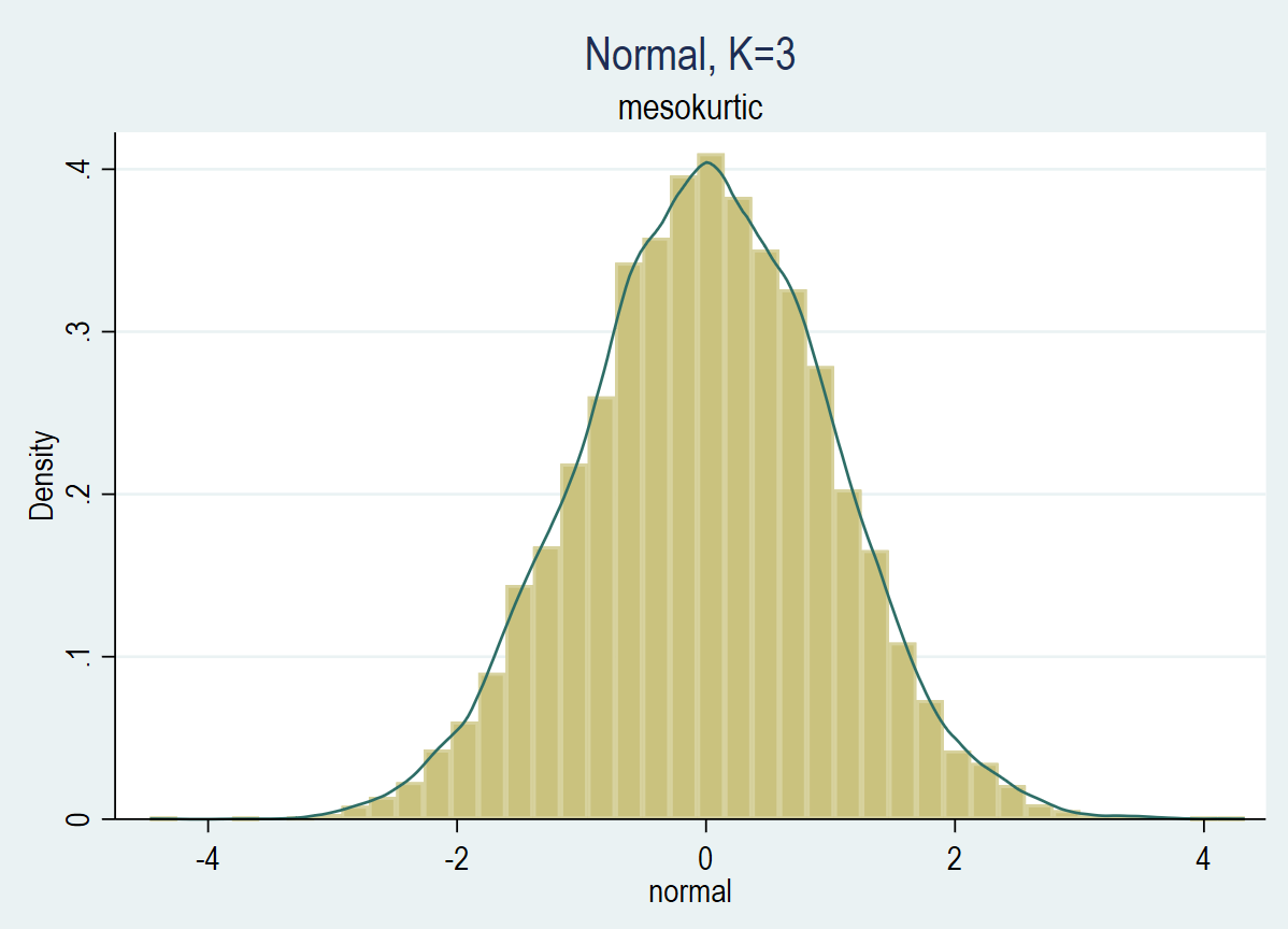
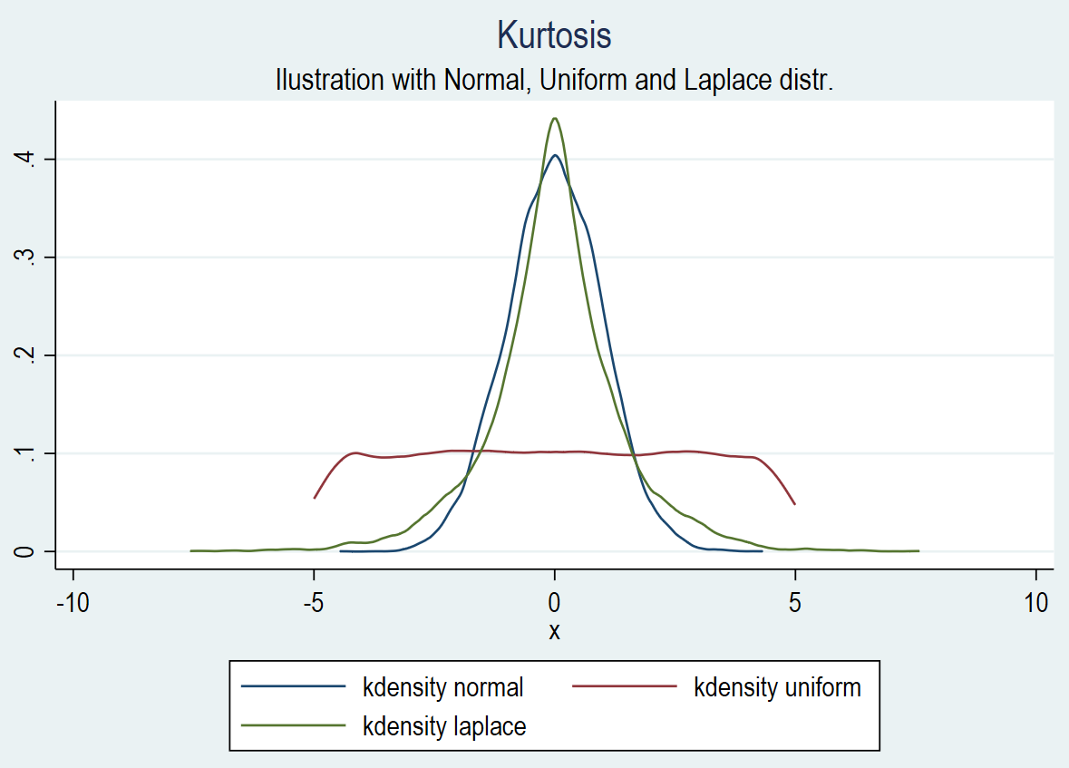
g_{2}=\frac{m_{4}}{m_{2}^{2}}= \frac{ \frac{1}{n}\sum_{i=1}^{n}(x_{i}-\bar{x})^{4} }{ [\frac{1}{n}\sum_{i=1}^{n}(x_{i}-\bar{x})^{2}]^{2} } \\

The kurtosis for a random variable that follows a Normal distribution is 3 (the ratio between the fourth moment and the square of the second moment, 3/(1^2)=3). We have a mesokurtic distribution. In figure 1, we have a distribution with the usual properties for a normal distribution:

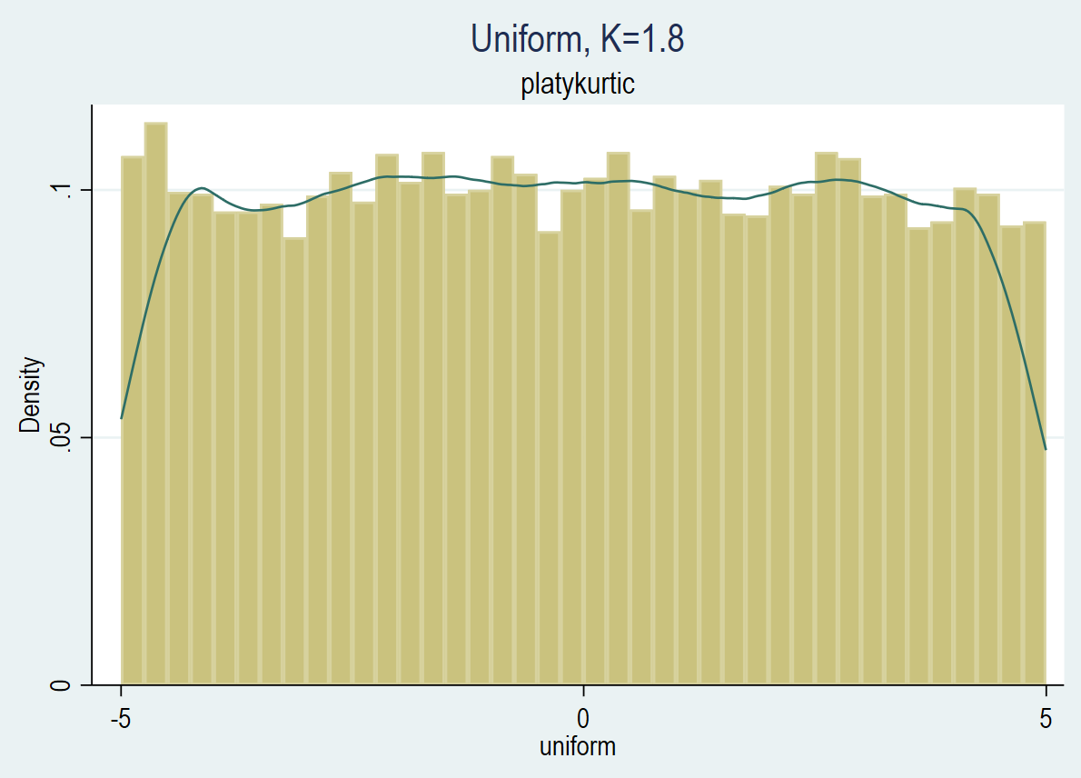
The kurtosis for a random variable that follows a Uniform distribution is below 3 (the ratio between the fourth moment and the square of the second moment, 125/(25/3)^2=1.8). We have a platykurtic distribution. In figure 2, we have a distribution with thinner tails than a normal distribution:

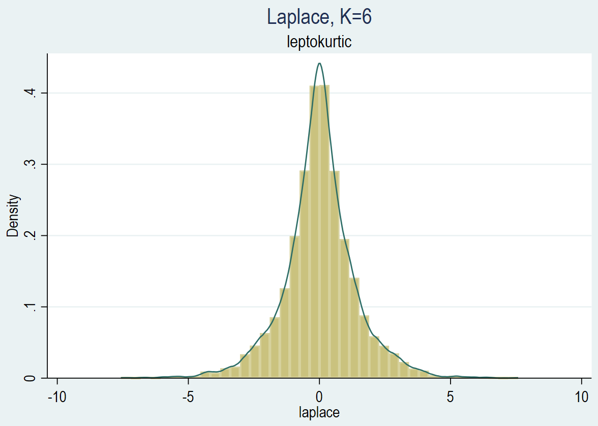
The kurtosis for a random variable that follows a Laplace distribution is above 3 (the ratio between the fourth moment and the square of the second moment, 24/(2^2)=6). We have a leptokurtic distribution. In figure 3, we have a distribution with thicker tails than a normal distribution:

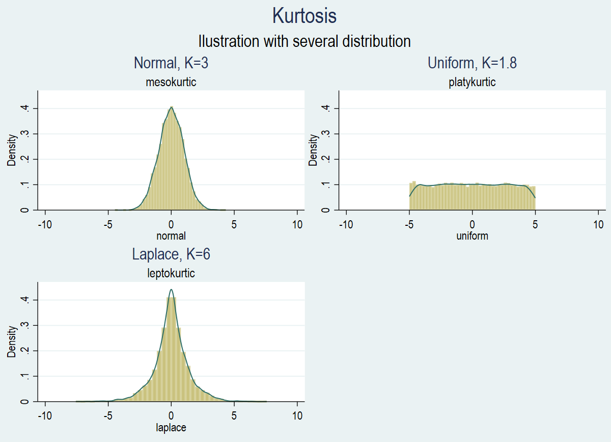
We can combine figures 1 to 3 to compare the kurtosis in figure 4:

We can superpose the three kernel density estimations in order to have a better view of the distributions respective thickness of the distribution’s tail:

The STATA code used to produce the graphs is reproduced below:

* Illustrate the Kurtosis
*------------------------

version 15.1
set more off
capture log close
cd ... // Replace with your own path                            
log using kurtosis, name(kurtosis) text replace

// Apply the s2color scheme

set scheme s2color

// Generate random variables

set obs 10000

// Normal variable

capture gen normal = rnormal()

sum normal, detail

// Uniform variable

capture gen uniform = runiform(-5,5)

sum uniform, detail

// Laplace variable

capture gen laplace = rlaplace(0,1)

sum laplace, detail

histogram normal, title("Normal, K=3") ///
subtitle(mesokurtic) kdensity

capture graph rename normal, replace
capture graph export normal.png, replace

histogram uniform, title("Uniform, K=1.8") ///
subtitle(platykurtic) kdensity

capture graph rename uniform, replace
capture graph export uniform.png, replace

histogram laplace, title("Laplace, K=6") ///
subtitle(leptokurtic) kdensity

capture graph rename laplace, replace
capture graph export laplace.png, replace

graph combine normal uniform laplace, ///
ycommon xcommon imargin(zero) ///
title(Kurtosis) ///
subtitle("Ilustration with several distribution")

capture graph rename kurtosis, replace
capture graph export kurtosis.png, replace

twoway (kdensity normal) (kdensity uniform) (kdensity laplace), ///
title(Kurtosis) ///
subtitle("Ilustration with Normal, Uniform and Laplace distr.")

capture graph rename kurtosis_gathered, replace
capture graph export kurtosis_gathered.png, replace

// Save the data
save ///
"kurtosis.dta", ///
replace // Note 1

log close
exit

Description
-----------

This file aims at illustrating the kurtosis.

Note :
------
1)  Replace the "..." by the path of the current directory.