Teaching sometimes generates new research results. During the Timberlake training, Local Projections for Time-Series and Panel Data Analysis, the students and I revisited the buffer effect documented in Aizenman et al. (2024). We first reproduced the panel local projections with locproj and then examined whether the same economic conclusion survived with the split-panel jackknife estimator implemented in the recently updated xtlp package.
This new exercise became possible because the latest version of xtlp substantially expands the command’s inference options. It implements the split-panel jackknife estimator directly and now supports heteroskedasticity-robust, one- and two-way cluster-robust, and Driscoll-Kraay covariance estimators. The SPJ correction and Driscoll-Kraay inference can therefore be combined inside a single xtlp call, without the manual workaround previously required.
Why the real-exchange-rate response has no predetermined sign
A terms-of-trade shock is a change in an international relative price, not a direct exchange-rate shock. It changes national purchasing power, the relative profitability of domestic sectors, consumption choices and the demand for external finance. The real exchange rate is the price that helps reconcile all of those adjustments. Its response is therefore determined by several mechanisms that need not point in the same direction.
1. What exactly is the terms-of-trade shock?
The terms of trade compare an economy’s export-price index with its import-price index:
\[ TOT_t=\frac{P_{X,t}}{P_{M,t}}, \qquad tot_t=\log(TOT_t). \]An increase is an improvement: a given volume of exports can purchase a larger volume of imports. But the ratio alone does not identify the origin of the movement. The same improvement can result from \(P_X\uparrow\), \(P_M\downarrow\), or unequal movements in both prices. These cases have different effects on export revenue, imported-input costs, consumer prices and sectoral profitability.
The paper also accounts for the fact that a given price movement matters more for a highly open economy. It constructs effective terms of trade by interacting the log terms of trade with trade exposure:
\[ to_t=\log\!\left(1+\frac{X_t}{Y_t}+\frac{M_t}{Y_t}\right), \qquad etot_t=to_t\times tot_t. \]Thus, etot combines the international price change with the economy’s exposure to trade. This scaling improves the economic relevance of the shock, but it does not by itself make the shock structural or determine the sign of its effect.
2. Which real exchange rate is adjusting?
Under the convention used in the paper, an increase in lreer denotes a real appreciation. For bilateral intuition, let \(E_t\) be the amount of foreign currency obtained for one unit of domestic currency. A price-based real exchange rate can then be written as:
The empirical REER is the trade-weighted counterpart of this expression. It can appreciate because the nominal currency strengthens, because domestic prices rise relative to foreign prices, or because the composition of domestic prices changes. In small-open-economy models, particular attention is paid to the internal relative price \(P_N/P_T\), where \(P_N\) is the price of nontradable goods and \(P_T\) is a tradable-goods price index. A rise in \(P_N/P_T\) usually contributes to a real appreciation, but this internal relative price is one component of the measured REER, not its definition.
For example, if the tradable price index is a geometric average of export and import prices,
\[ P_T=P_X^{\omega}P_M^{1-\omega}, \qquad 0<\omega<1, \]then its contribution to the internal real exchange rate satisfies:
\[ d\log\!\left(\frac{P_N}{P_T}\right) = d\log P_N -\omega\,d\log P_X -(1-\omega)\,d\log P_M. \]This identity makes two points explicit. First, \(P_N\) is endogenous and must respond to domestic demand and supply. Second, an export-price increase and an import-price decrease enter the tradable price index differently even when they produce the same change in \(TOT\).
3. A three-good way to organize the mechanisms
Consider a small economy that produces an exportable good \(X\) and a nontradable good \(N\), and consumes an importable good \(M\) together with \(N\). World markets determine \(P_X\) and \(P_M\), while \(P_N\) must clear the domestic market. In a deliberately compact notation, equilibrium for nontradables is:
\[ D_N\!\left(\frac{P_N}{P_M},Y\right) = S_N\!\left(\frac{P_N}{P_X};K,L\right). \]A terms-of-trade improvement changes the income term \(Y\), the consumer price of imports relative to nontradables, and the profitability of producing exports relative to nontradables. It therefore shifts both sides of this market-clearing condition. After normalizing by the positive own-price response that restores equilibrium, the sign can be summarized schematically as:
\[ \frac{d\log(P_N/P_T)}{d\log(TOT)} = \underbrace{\mathcal I}_{\text{income/spending}} + \underbrace{\mathcal C}_{\text{consumption substitution}} + \underbrace{\mathcal R}_{\text{production reallocation}}. \]If nontradables are normal goods, \(\mathcal I\) normally points toward appreciation. The signs of \(\mathcal C\) and \(\mathcal R\) depend on substitution elasticities, factor mobility and the origin of the shock. This is a conceptual decomposition rather than the estimating equation used below.
4. The income or spending effect
A favorable terms-of-trade shock increases real national income relative to domestic production. Higher export prices raise the purchasing power of export receipts; lower import prices allow households, firms and the government to obtain more foreign goods for the same expenditure. If part of this gain is spent on domestic services, housing, construction and other nontradables, demand for \(N\) rises.
Holding traded quantities fixed, the first-order purchasing-power gain can be represented approximately as:
\[ dY_t^{d} \simeq \bar X_t\,dP_{X,t} – \bar M_t\,dP_{M,t}, \]where \(\bar X_t\) and \(\bar M_t\) are export and import volumes. The expression is positive after either an export-price increase or an import-price decrease, but it says nothing yet about how the additional income is spent or how domestic production responds.
Unlike imports, nontradables cannot be supplied from the world market at a fixed international price. Their market must clear domestically. When their short-run supply is inelastic, much of the additional demand is absorbed through a higher \(P_N\), wages and rents rather than through output. This is the classic spending effect: \(P_N/P_T\) rises and the real exchange rate appreciates. The effect is stronger when the beneficiaries of the windfall have a high propensity to spend domestically, when government consumption is intensive in nontradables, and when the nontradable supply response is slow.
The size of the income effect also depends on trade exposure, ownership and distribution. A world-price increase creates little domestic income when the relevant export sector is small or largely foreign-owned and profits are repatriated. Conversely, a concentrated commodity boom can have a large fiscal effect when the government captures export rents and spends them locally.
5. Consumption substitution and production reallocation
An increase in export prices. When \(P_X\) rises, producing the exportable becomes more profitable. Mobile labor and capital may move from nontradables toward the booming export sector. If this reduces the supply of nontradables, \(P_N\) rises. The resulting resource-movement effect reinforces the spending effect and produces appreciation in the benchmark Dutch-disease model of Corden and Neary (1982).
This result is not universal. Factor specificity can limit movement between sectors. Export production may use nontradable services as complements, increasing their demand, or it may release factors that expand their supply. The export sector may also use imported intermediate inputs much more intensively than the rest of the economy. These production linkages determine whether the supply of nontradables contracts or expands after the shock.
A decrease in import prices. When \(P_M\) falls, real purchasing power rises, so the income effect still tends to increase demand for nontradables. At the same time, imports become cheaper relative to domestic goods. Consumers may substitute imported goods for locally produced goods, reducing demand for \(N\). Firms using imported machinery, energy or intermediate inputs experience lower marginal costs; if nontradable producers are import-intensive, their supply expands and \(P_N\) falls. These consumption and cost channels generate depreciation pressure and may dominate the favorable income effect.
The relative strength of the mechanisms depends on whether goods are substitutes or complements in consumption and production. Tokarick (2008) shows formally that the relative price of nontradables can rise or fall following a terms-of-trade improvement. If nontradables are net substitutes for the export good, the substitution effect may reinforce the income effect; with different cross-price relationships, it may offset or overturn it.
6. Export-price and import-price shocks are not mirror images
A 10% rise in export prices and an approximately 9.1% fall in import prices generate the same proportional improvement in \(P_X/P_M\), but they are economically distinct. The first directly raises export-sector revenue and profitability; the second directly lowers consumer prices and production costs. Countries also have different export concentration, import composition and exposure to commodity prices. An aggregate terms-of-trade index compresses these differences into a single ratio.
Di Pace, Juvenal and Petrella (2025) show empirically that positive export-price shocks do not mirror negative import-price shocks. Export-price shocks tend to have larger and more persistent effects in developing economies. Their analysis also shows why the ratio can conceal relevant global shocks: export and import prices may move together, leaving \(TOT\) almost unchanged even though both movements affect domestic activity and the REER.
7. Persistence, saving and the current account
The response also depends on whether the shock is temporary, persistent or anticipated. A household that smooths consumption reacts to a temporary windfall by saving a substantial part of it; current absorption and nontradable demand then rise by less than current income. A persistent improvement changes lifetime resources more strongly and generally supports a larger response of consumption, investment and wages. Anticipated future changes can affect spending before the observed terms of trade move.
The traditional Harberger-Laursen-Metzler argument links a deterioration in the terms of trade to lower real income, lower saving and a weaker current account. Intertemporal models show that this conclusion is not automatic. Svensson and Razin (1983) demonstrate that the response depends on the timing and expected duration of the shock, while Obstfeld (1982) shows that a permanent deterioration can reduce aggregate spending and generate a current-account surplus in an optimizing model. These are current-account results rather than direct REER theorems, but they matter here because saving determines how much of the income change reaches domestic nontradable demand.
Financial development changes this intertemporal margin. Deep credit, insurance and hedging markets allow households and firms to smooth external shocks privately. Where financial institutions are weak, borrowing constraints and limited risk sharing make domestic expenditure more sensitive to cash flow and external financing conditions. Public reserves can then substitute partly for missing private insurance, which provides the economic rationale for the threshold result studied in the paper.
8. Nominal adjustment, fiscal policy and reserves
Under a floating exchange-rate regime, the nominal currency can respond quickly to news about export income, capital flows and future monetary conditions. A favorable shock may produce a nominal appreciation before domestic quantities or prices adjust. Under a peg, the nominal channel is constrained, so adjustment occurs more through domestic inflation, wages, output and reserve flows. The observed response also depends on exchange-rate pass-through: a nominal movement has a larger immediate effect on domestic tradable prices when pass-through is high.
Fiscal policy determines how much of the windfall becomes domestic absorption. Saving export revenue in foreign assets or a sovereign wealth fund limits demand for nontradables; spending it on public wages and locally produced services strengthens appreciation pressure. Monetary policy matters as well: an inflation-targeting central bank may offset domestic price pressure, whereas accommodation may allow a larger increase in \(P_N\).
Reserve management affects both the size and timing of adjustment. During a favorable external shock, the central bank can purchase foreign currency and accumulate reserves, leaning against nominal appreciation and transferring part of the windfall abroad. During an adverse shock, it can sell reserves to support the currency, finance essential imports and smooth domestic expenditure. Sterilization is important: an unsterilized reserve purchase expands domestic liquidity and may raise domestic prices, partly offsetting the nominal-exchange-rate effect. Aizenman and Riera-Crichton (2008) and Aizenman, Edwards and Riera-Crichton (2012) provide direct evidence on this reserve-buffer channel.
9. Putting the channels together
| Channel | Appreciation pressure | Depreciation or attenuation |
|---|---|---|
| Income and spending | The windfall is spent on supply-constrained nontradables. | The gain is saved abroad, repatriated, or spent mainly on imports. |
| Consumption substitution | Expenditure shifts toward domestic nontradables. | Cheaper imports displace domestic demand. |
| Production reallocation | The export boom draws factors out of nontradables and reduces their supply. | Cheaper imported inputs expand domestic supply or factor mobility is limited. |
| Persistence and finance | A persistent gain raises lifetime wealth and current absorption. | A temporary gain is smoothed through saving and external assets. |
| Nominal exchange rate | A floating currency appreciates and pass-through is rapid. | A peg or intervention delays the nominal adjustment. |
| Fiscal and reserve policy | The windfall finances domestic government expenditure. | Fiscal saving, sterilized intervention and reserve accumulation absorb it. |
There is consequently no sign a priori for the total REER response. De Gregorio and Wolf (1994) and Mendoza (1995) provide influential models and evidence in which appreciation-producing forces dominate. Cashin, Céspedes and Sahay (2004) find substantial heterogeneity across commodity exporters. These results are empirical regularities or model outcomes, not a theoretical restriction.
In Aizenman et al. (2024), the direct coefficient on effective terms of trade is positive in the baseline regression. This means that appreciation-producing channels dominate on average in that sample; it does not identify the income effect separately from substitution, production, nominal or policy channels. The negative interaction with lagged reserves then says that a larger pre-shock reserve buffer reduces that estimated slope. The distinction is essential: the direct response is an empirical result, whereas the reserve interaction describes how the response changes with reserves.
The buffer effect
In the paper’s baseline estimates, the direct terms-of-trade coefficient is positive. This means that appreciation-producing channels dominate depreciation-producing channels on average in the sample; the regression does not separately identify the income, substitution and production mechanisms. The sign is estimated rather than imposed. In a dynamic interaction specification, the marginal response at horizon \(h\) can be written as:
\[ \frac{\partial \ell REER_{i,t+h}}{\partial\,\Delta etot_{i,t}} =\theta_h+\beta_h R_{i,t-1}, \]where \(R_{i,t-1}\) is the reserve buffer before the shock. Equivalently, the interaction coefficient is the cross-partial derivative:
\[ \frac{\partial^2 \ell REER_{i,t+h}} {\partial\,\Delta etot_{i,t}\,\partial R_{i,t-1}} =\beta_h. \]A negative \(\beta_h\) makes the response less positive—or more negative—as reserves rise. It is a buffer against appreciation when the direct response \(\theta_h\) is positive; the interaction coefficient alone does not determine the sign of the total response.
In the estimator comparison below, the impulse is instead the interaction between residualized changes in terms of trade and reserves, denoted by \(S_{i,t}\). At each annual horizon \(h\), the robustness regression is summarized by:
\[ \ell REER_{i,t+h} = \alpha_i^{(h)} + \rho_h \ell REER_{i,t-1} + \beta_h S_{i,t} + \Gamma_h^{\prime}X_{i,t-1} + \varepsilon_{i,t+h}. \]What are the residualized variables?
The impulse \(S_{i,t}\) is constructed before estimating the local projections. The code first uses Stata’s first-difference operator D. and runs two OLS regressions with country indicators:
Here, \(lres\) is the logarithmic reserve measure, \(etot\) is effective terms of trade, and \(\eta_i\) denotes the country fixed effects implemented by cny*. The corresponding Stata commands are:
reg D.lres lreer cny* if count_lgovexp == 20, robust
predict residuals_lres, residuals

reg D.etot lreer cny* if count_lgovexp == 20, robust
predict residuals_etot, residuals
residuals_lres is therefore the part of the annual change in log reserves that is not linearly explained by the contemporaneous real exchange rate or permanent country characteristics. Likewise, residuals_etot is the unexplained part of the annual change in effective terms of trade. In the first-stage estimation sample, each residual is orthogonal by construction to lreer and the included country indicators.
The LP impulse is their product:
\[ S_{i,t} = \widehat{u}_{i,t}^{e}\widehat{u}_{i,t}^{r} = residuals\_etot_{i,t}\times residuals\_lres_{i,t}. \]This is not a shock to terms of trade alone. It is a one-unit increase in the interaction between the residualized changes in effective terms of trade and reserves. A positive value can arise when both residual changes have the same sign; a negative value arises when they have opposite signs. The residualization targets one specific reverse-causality concern by removing the linear variation in each component associated with the current real exchange rate. It is a robustness device, not a claim that the interaction is a fully identified structural shock.
Because an increase in the log real effective exchange rate denotes an appreciation, \(\beta_h<0\) means that a larger value of this interaction shifts the real-exchange-rate response downward. When the direct terms-of-trade response is an appreciation, this negative interaction is the buffer effect: reserve adjustment reduces the magnitude of that appreciation. It should not be interpreted as imposing a positive direct terms-of-trade effect in advance.
First result: locproj
The figure below reports the estimates produced with locproj, using met(xtscc). It is therefore a graphical presentation of the conventional fixed-effects panel local projections with Driscoll-Kraay inference. It does not report the subsequent xtlp estimates.
The three panels convey a clear qualitative pattern. The response is negative in the full sample and becomes more persistent below the financial-institution threshold. Above the threshold, the estimates are much less precise and the confidence intervals cover zero throughout.
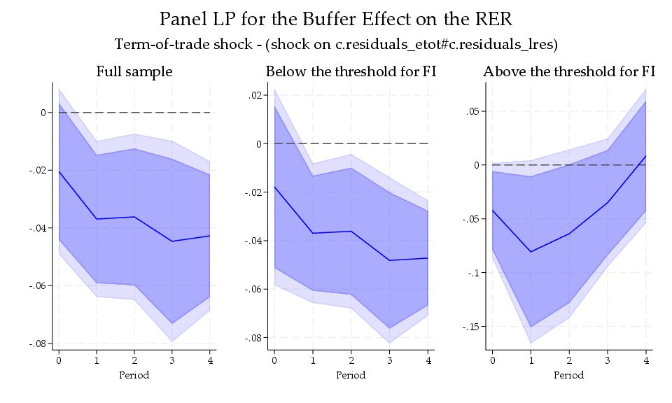
locproj. Panel local projections for the buffer effect on the real exchange rate. The sample is divided using the previously estimated financial-institution threshold of approximately 0.48. The dark and light shaded areas report 90% and 95% confidence intervals, respectively.Second result: xtlp with the SPJ correction
As an additional robustness exercise, we re-estimated the dynamic responses with xtlp. These regressions use country fixed effects, the split-panel jackknife (SPJ) correction and Driscoll-Kraay standard errors with two lags. The SPJ correction is useful here because the model combines a lagged dependent variable with a relatively short time dimension. Driscoll-Kraay inference allows for serial dependence over time and cross-sectional dependence among countries.
The following command shows the full-sample specification. We then re-estimated it for observations with L2.fi<0.48 and L2.fi>=0.48.
xtlp lreer ///
    (c.residuals_etot#c.residuals_lres) ///
    L.lreer ///
    (L.lgdppk_m100 L.lgovexp L.irr), ///
    fe method(spj) hor(4) ytransf(level) ///
shock(1) vce(dk lag(2), ase) g| Horizon | Full sample | FI below 0.48 | FI at or above 0.48 |
|---|---|---|---|
| 0 | -0.046 | -0.027 | 0.057 |
| 1 | -0.055* | -0.039* | 0.021 |
| 2 | -0.055* | -0.068* | -0.009 |
| 3 | -0.049* | -0.077* | 0.031 |
| 4 | -0.046* | -0.079* | -0.010 |
* The 95% confidence interval excludes zero.
The xtlp results confirm the same pattern. In the full sample, the response is negative and statistically significant from one to four years. Below the financial-institution threshold, it becomes progressively stronger, moving from -0.039 after one year to -0.079 after four years. Above the threshold, the point estimates fluctuate around zero and none is statistically significant.
We also checked the inference with two-way clustering by country and year. Clustering by country allows arbitrary correlation of the disturbances over time within a country, whereas clustering by year allows arbitrary contemporaneous correlation across countries exposed to the same global shocks. This alternative produced results similar to those obtained with Driscoll-Kraay standard errors: the response remains negative and persistent in the full sample and below the financial-institution threshold, while it remains statistically indistinguishable from zero above the threshold. The conclusion is therefore robust to both approaches to dependence in the panel.
The numerical values in Figure 1 and Table 1 should not be read as if they came from the same estimator. Figure 1 contains the locproj estimates, whereas Table 1 contains the SPJ-corrected xtlp estimates. SPJ changes the point estimation, and the effective sample can also change across horizons when singleton observations are removed. The relevant robustness result is that both approaches deliver the same qualitative conclusion.
International reserves provide a more important buffer when financial institutions are comparatively underdeveloped. This exercise takes the threshold previously estimated in the paper as given; it is an estimator-based robustness check, not a new test of the threshold itself.
It was also a valuable illustration of how teaching and research can reinforce one another: the additional xtlp result emerged directly from empirical work with the students during the Timberlake training.
References
Aizenman, J., Ho, S.-H., Huynh, L. D. T., Saadaoui, J., and Uddin, G. S. (2024). “Real exchange rate and international reserves in the era of financial integration.” Journal of International Money and Finance, 141, 103014. https://doi.org/10.1016/j.jimonfin.2024.103014.
Aizenman, J., and Riera-Crichton, D. (2008). “Real exchange rate and international reserves in an era of growing financial and trade integration.” The Review of Economics and Statistics, 90(4), 812–815. https://doi.org/10.1162/rest.90.4.812.
Aizenman, J., Edwards, S., and Riera-Crichton, D. (2012). “Adjustment patterns to commodity terms-of-trade shocks: The role of exchange rate and international reserves policies.” Journal of International Money and Finance, 31(8), 1990–2016. https://doi.org/10.1016/j.jimonfin.2012.05.003.
Cashin, P., Céspedes, L. F., and Sahay, R. (2004). “Commodity currencies and the real exchange rate.” Journal of Development Economics, 75(1), 239–268. https://doi.org/10.1016/j.jdeveco.2003.08.005.
Corden, W. M., and Neary, J. P. (1982). “Booming sector and de-industrialisation in a small open economy.” The Economic Journal, 92(368), 825–848. https://doi.org/10.2307/2232670.
De Gregorio, J., and Wolf, H. C. (1994). “Terms of trade, productivity, and the real exchange rate.” NBER Working Paper No. 4807. https://doi.org/10.3386/w4807.
Di Pace, F., Juvenal, L., and Petrella, I. (2025). “Terms-of-trade shocks are not all alike.” American Economic Journal: Macroeconomics, 17(2), 24–64. https://doi.org/10.1257/mac.20220035.
Mendoza, E. G. (1995). “The terms of trade, the real exchange rate, and economic fluctuations.” International Economic Review, 36(1), 101–137. https://doi.org/10.2307/2527429.
Obstfeld, M. (1982). “Aggregate spending and the terms of trade: Is there a Laursen-Metzler effect?” The Quarterly Journal of Economics, 97(2), 251–270. https://doi.org/10.2307/1880757.
Svensson, L. E. O., and Razin, A. (1983). “The terms of trade and the current account: The Harberger-Laursen-Metzler effect.” Journal of Political Economy, 91(1), 97–125. https://doi.org/10.1086/261130.
Tokarick, S. (2008). “Commodity currencies and the real exchange rate.” Economics Letters, 101(1), 60–62. https://doi.org/10.1016/j.econlet.2008.04.008.