Using addplot to make high-quality graph with Stata (May 2025)

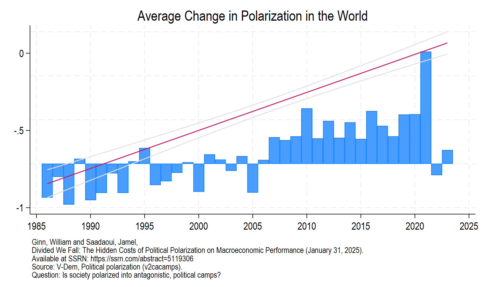
For an ongoing project on political polarization with William Ginn, I have to make a graph to explain how evolve political polarization around the world. Fortunately, I found a very useful feature in Stata to add plots to existing graphs. We are going to reproduce the following figure:

You have to install the package written by Ben Jann:

https://github.com/benjann/addplot
https://ideas.repec.org/c/boc/bocode/s457917.html

Let us start with by examining the code:

gen Dv2cacamps=D.v2cacamps
bys year: egen Dv2cacampsM=mean(Dv2cacamps)

tw ///
 bar Dv2cacampsM year if Dv2cacampsM!=. ///
 , xlabel(1985(5)2025) name(W, replace) ///
 ti("Average Change in Polarization in the World") ///
 , yti("") xti("") legend(off) ///
 note("Ginn, William and Saadaoui, Jamel," ///
 "Divided We Fall: The Hidden Costs of Political Polarization on Macroeconomic Performance (January 31, 2025)." ///
 "Available at SSRN: https://ssrn.com/abstract=5119306" ///
 "Source: V-Dem, Political polarization (v2cacamps)." ///
 "Higher values indicate higher polarization.")
 
 addplot: lfitci v2cacamps year if Dv2cacampsM!=. ///
  , yaxis(2) yscale(off) ciplot(rline) xlabel(1985(5)2025)

The first part in bold is quite standard and produces the following graph:

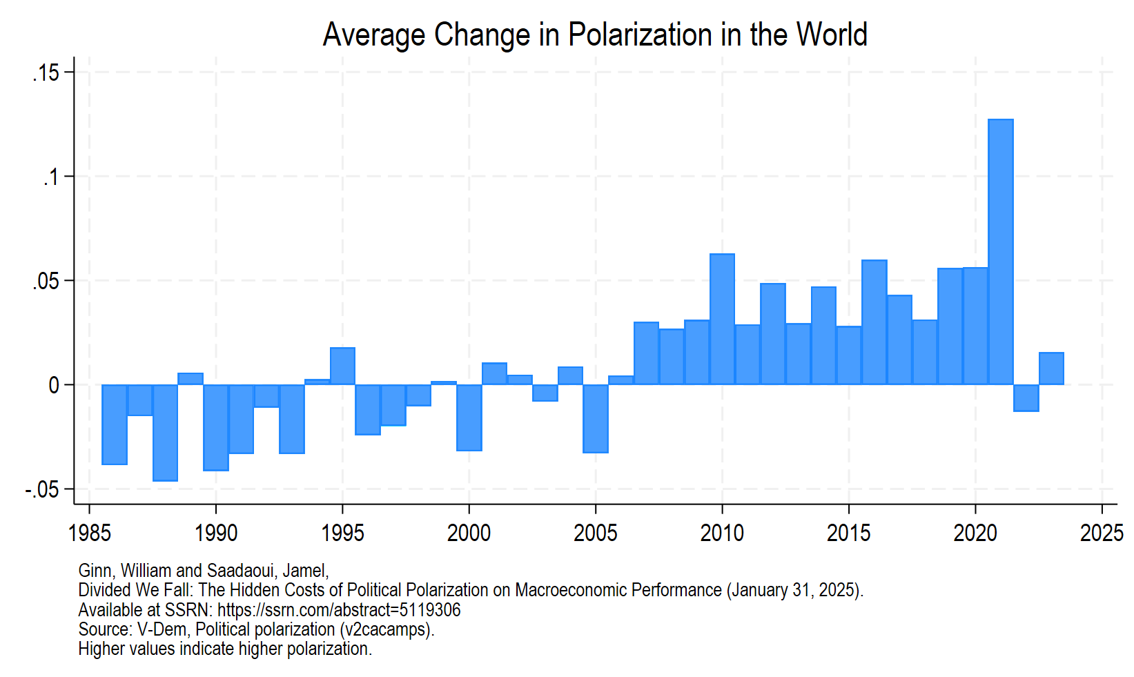
The second part allows you to add the estimates and the confidence intervals for a simple regression of mean polarization on a time trend. You can remove the yaxis for the superposed graph:

tw ///
 bar Dv2cacampsM year if Dv2cacampsM!=. ///
 , xlabel(1985(5)2025) name(W, replace) ///
 ti("Average Change in Polarization in the World") ///
 , yti("") xti("") legend(off) ///
 note("Ginn, William and Saadaoui, Jamel," ///
 "Divided We Fall: The Hidden Costs of Political Polarization on Macroeconomic Performance (January 31, 2025)." ///
 "Available at SSRN: https://ssrn.com/abstract=5119306" ///
 "Source: V-Dem, Political polarization (v2cacamps)." ///
 "Higher values indicate higher polarization.")
 
 addplot: lfitci v2cacamps year if Dv2cacampsM!=. ///
  , yaxis(2) yscale(off) ciplot(rline) xlabel(1985(5)2025)

Overall, this a very handy command. The working paper is available here:
https://papers.ssrn.com/sol3/papers.cfm?abstract_id=5119306

The following blog is also susceptible to arouse your curiosity: