After three blogs on how to draw maps with Stata for the NUTS regions and on how to download data from DBnomics, this time I will show you how to draw bivariate maps for the wage variations and unemployment gaps in the NUTS 2 regions:
First, I will use the solution provided by Scott Merryman on the Stata list to superpose different maps:
spshape2dta  nuts_rg_03m_2021_3035_levl_2, replace

use  nuts_rg_03m_2021_3035_levl_2.dta,clear
drop if _CX < 2100000
drop if _CY <0
save, replace

//test
spmap using  nuts_rg_03m_2021_3035_levl_2_shp, id(_ID) ///
 ocolor(blue ) os(vthin) ///
 polygon(data(nuts_rg_03m_2021_3035_levl_2_shp) osize(thin)) ///
 name(nuts0_2,replace)


spshape2dta  nuts_rg_03m_2021_3035_levl_0, replace
use  nuts_rg_03m_2021_3035_levl_0_shp,clear
drop if _X <  2100000
drop if _Y < 0
gen nuts = 2
save,replace

// use nuts_rg_01m_2016_3035_levl_0.dta,clear
// spmap using  nuts_rg_01m_2016_3035_levl_0_shp, id(_ID)

spshape2dta  nuts_rg_03m_2021_3035_levl_1, replace
use nuts_rg_03m_2021_3035_levl_1.dta,clear
drop if _CX < 2000000
save, replace

use nuts_rg_03m_2021_3035_levl_1_shp
drop if _X <  2100000
drop if _Y < 0
gen nuts = 1
append using nuts_rg_03m_2021_3035_levl_0_shp
save,replace

use nuts_rg_03m_2021_3035_levl_2.dta
spmap using  nuts_rg_03m_2021_3035_levl_2_shp, id(_ID) ///
 ocolor(blue ) os(vthin) ///
 polygon(data(nuts_rg_03m_2021_3035_levl_1_shp) by(nuts) ///
 osize(vthin ..) ocolor(red black ))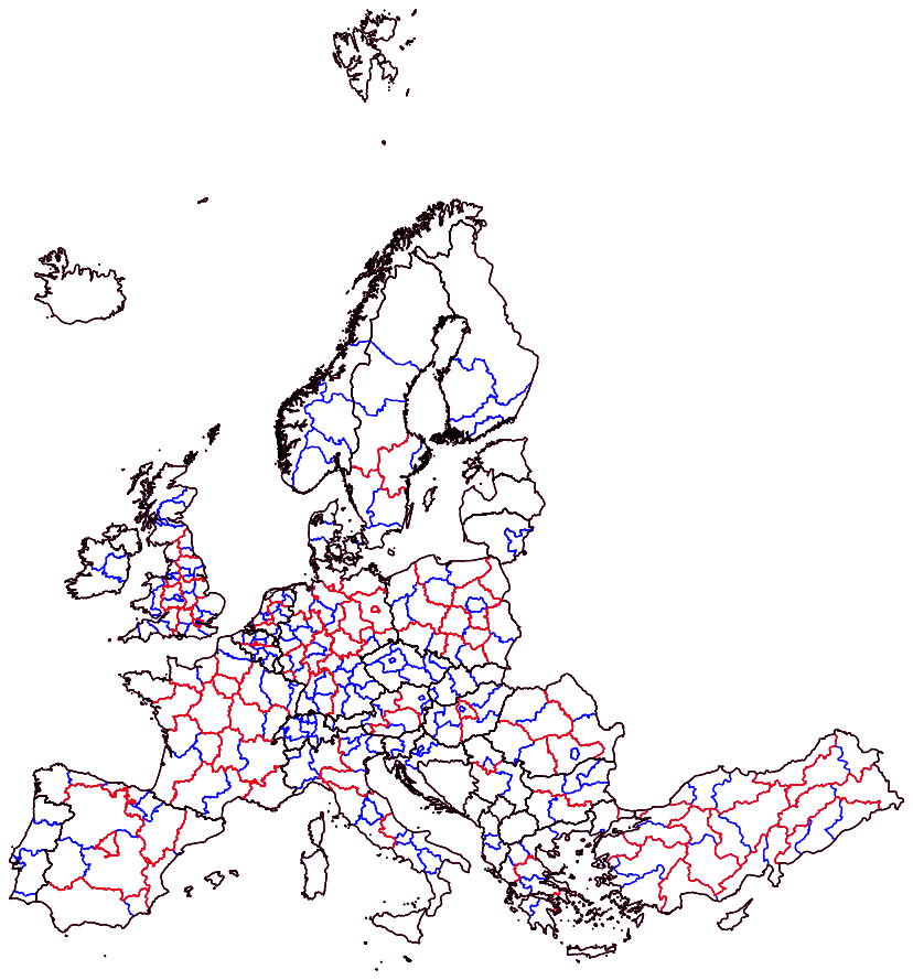
Then, you have to follow the steps that are explained in a previous post on Chinese provinces:
use PCurve_NUTS2.dta, clear

decode GEO, gen(NUTS_ID)

xtset GEO period

gen HWAGE = log(1000*(COMP/HOURS))
gen DHWAGE = d.HWAGE

sum HWAGE DHWAGE UNEMP_cycle

winsor2 DHWAGE, suffix(_w) cuts(5 95) by(period)

sum HWAGE DHWAGE DHWAGE_w

** HAMILTON FILTER **
hamiltonfilter UNEMP, stub(UNEMP) frequency(yearly)

format DHWAGE UNEMP %4.2f

save PCurve_NUTS2maps.dta, replace

use nuts_rg_03m_2021_3035_levl_2.dta

foreach v in PCurve_NUTS2maps {
		     merge 1:m NUTS_ID using `v'.dta
}

// Run everything from here
set scheme white_tableau

forvalues v = 2018(1)2019 {
replace period=`v' if _merge==1
bimap DHWAGE UNEMP_cycle using ///
 nuts_rg_03m_2021_3035_levl_2_shp if period==`v' ///
 , cut(pctile) formaty(%4.2f) ///
 palette(bluered)  ///
 title("{fontface STIX Two Text Bold:Bivariate Map of Wage and Unemployment Gap in `v'}") ///
 note("Note: NUTS 2 regions of EU members represented. Wage variation are windsorized") ///
 textx("Unemployment Gap") texty("Wage Variation") percent ///
 texts(3) textlabs(2.5) values ///
 ocolor(black) osize(0.025) ///
 ndfcolor(gray%30 ..) ndocolor(black ..) ///
 legend(pos(9) ring(0)) ///
 polygon(data("nuts_rg_03m_2021_3035_levl_0_shp") ///
 ocolor(black) osize(0.1))

graph rename Graph bimap`v', replace
graph export map`v'.png, as(png) width(4000) replace

}

**# End of Program 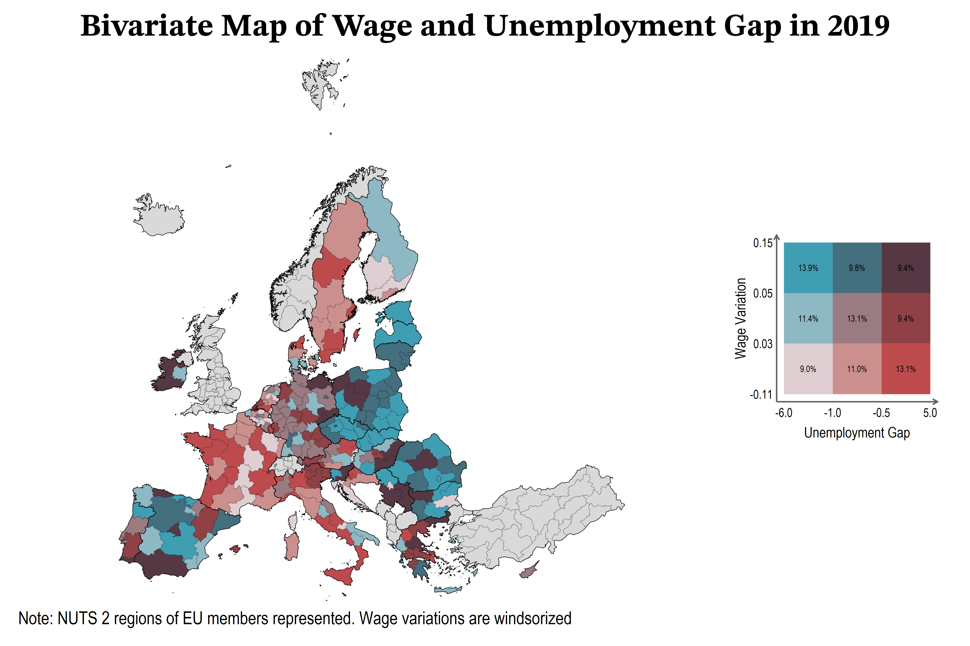
1 Comment
[…] Drawing bivariate maps with Stata for the NUTS regions (removing Turkey) […]