In a previous blog, I have shown how to estimate Panel VAR with the new command xtvar introduced in StataNow.
This time, I will use the EM-DAT database to estimate the impact of 630 large-scale natural disasters observed between 1990 and 2025 on the bond yields. I thank Evangelos Salachas for his help with the data. To create the dummy variable for the large-scale natural disasters, I follow Klomp (2015), which explains that: “investors perceive natural disasters as an adverse shock that makes the government debt less sustainable and eventually triggers a sovereign default.”
Klomp, J. (2015). Sovereign risk and natural disasters in emerging markets. Emerging Markets Finance and Trade, 51(6), 1326-1341, 10.1080/1540496X.2015.1011530.
Let us start with the estimation of the Panel VAR:
set scheme stcolor

xtdescribe

xtvar bonds_tw disaster, lags(3) maxldep(8) ///
fd collapse 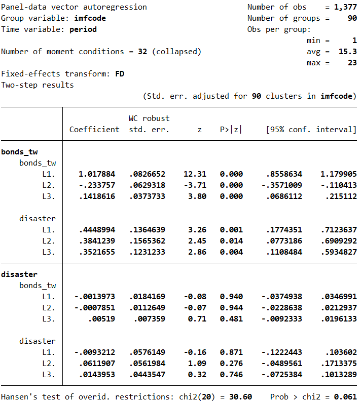
The model is over-identified (32 instruments for 12 parameters) and the over-identified restrictions are not rejected. I can test whether the VAR is stable. Besides, I can examine the Granger-causality:
varstable, ///
 graph name(stable, replace)

vargranger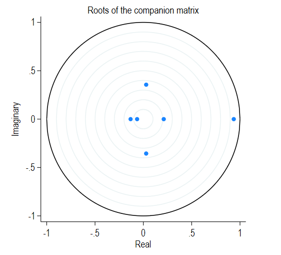
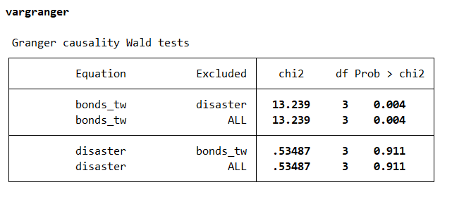
The Granger-causality runs from the large-scale natural disasters towards the bond yields (bonds_tw), since the p-values are below 1 percent in the upper panel.
We can plot the impulse response functions (IRF), after creating a dataset for the IRF:
irf create lags, ///
 set(example1) step(6) replace

irf graph irf, irf(lags) ///
 name(irf, replace)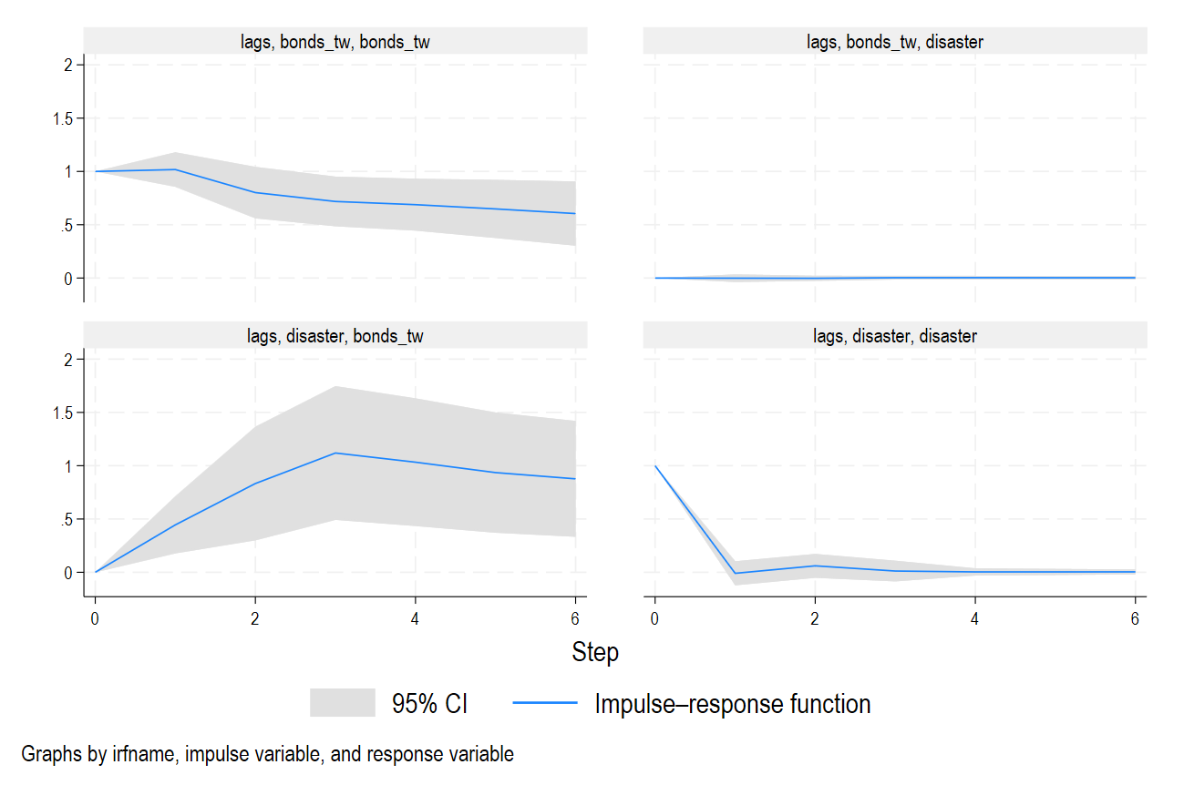
Finally, I can plot the orthogonalized impulse response functions (equivalent to the previous figure in a bivariate Panel VAR):
irf cgraph (lags disaster bonds_tw irf) ///
  (lags bonds_tw disaster irf), ///
  ycommon name(oirf, replace)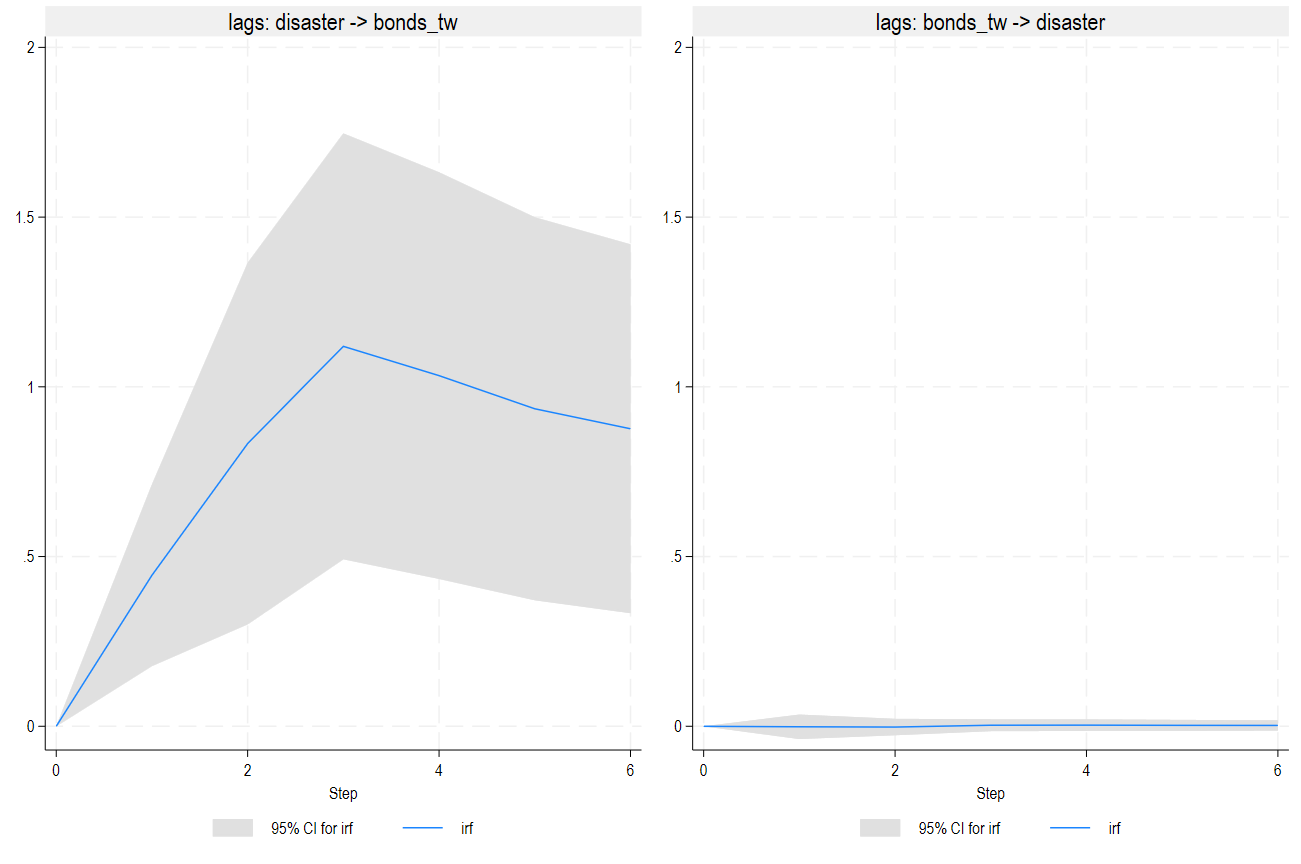
A large-scale natural disaster causes an increase in bond yields of 1 percent during multiple years.