In a previous blog, I showed how to draw local projection’s impulse response function with Driscoll-Kraay inference in Stata. This is the picture what you get:
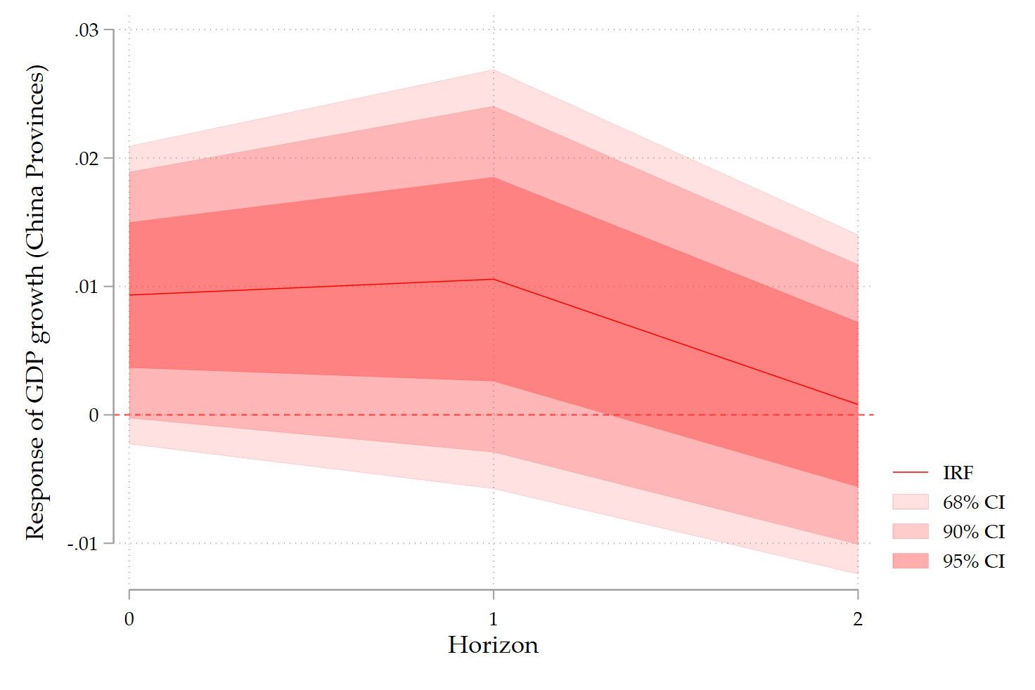
But, Alfonso Ugarte on LinkedIn told me that you can also use locproj to get a similar picture (while not yet documented in the locproj help):
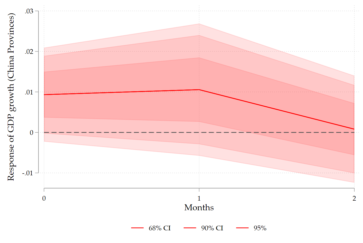
Full code below for pedagogical purposes:
foreach h in 68 90 95 {
   locproj D.GDP, shock(z_D_LUSA) ///
    h(2) yl(2) sl(0) zero ///
    c(L(1/2).(CPI TRADE GFCF POP TOT)) fe ///
    conf(`h') lcolor(sand) ///
    ttitle("Horizon") title(`"US-China"') ///
    noisily stats save irfname(iUS`h') grname(US`h') met(xtscc)
}

lpgraph iUS68 iUS90 iUS95, h(2) tti(Months) ///
  nolegend ///
  tti(Months) ti1(DK-LP) ///
  title("") ///
  lab1(68% CI) lab2(90% CI) lab3(95%) ///
  lc1(red) lc2(red) lc3(red) ///
  z grname(DK) grsave(DK) as(png) ///
  xtitle("Horizon") ///
  ytitle("Response of GDP growth (China Provinces)")