Do International Reserves Buffer Real-Exchange-Rate Adjustment after Terms-of-Trade Shocks? A Matching Application in Stata

This post illustrates how to use matching methods in Stata to study a reserve-buffer mechanism in international macroeconomics. The application uses kmatch, teffects, and a country-year panel to compare high- and low-reserve observations after large terms-of-trade disturbances.

1. Motivation

In my paper on real exchange rates and international reserves, the central mechanism is that reserves may act as a buffer. When a country is hit by a terms-of-trade shock, the real effective exchange rate may need to adjust. A high level of reserves can, in principle, dampen the size of that adjustment.

The baseline regression framework studies this mechanism through an interaction between effective terms of trade and lagged reserves:

areg lreer lgdppk_m100 lgovexp c.etot##c.L1lres yr* ///
    if count_lgovexp == 20, absorb(cn) vce(cluster cn)

This is a natural panel-data specification. But matching requires a binary treatment. The first temptation is to define a binary terms-of-trade shock and ask whether treated observations have different real exchange rates. That design is not ideal. The economic mechanism is not simply “high terms of trade cause high or low REER.” The mechanism is instead about whether reserves reduce the size of the exchange-rate response after an external disturbance.

This post therefore reformulates the matching design as follows:

Treatment: high lagged reserves.
Event sample: country-years hit by large absolute terms-of-trade shocks.
Outcome: the absolute cumulative real-exchange-rate response after the shock.
Interpretation: a negative ATT means that high reserves are associated with a smaller absolute REER adjustment.

This gives matching a clear economic interpretation: among country-years exposed to large terms-of-trade disturbances, compare high-reserve observations with otherwise similar low-reserve observations.

2. What matching does

Matching is an approach to condition on observed covariates. The idea is to find, for each treated observation, comparable control observations with similar pre-treatment characteristics. These controls are then used to construct the counterfactual outcome that the treated observation would have experienced without treatment.

In this application, the treatment is high lagged reserves. The counterfactual question is:

How large would the REER adjustment have been for high-reserve country-years after large terms-of-trade shocks if they had instead entered the shock with low reserves, holding observed pre-shock characteristics comparable?

The estimand is the average treatment effect on the treated:

ATT_h = E[Y_i,t+h(1) − Y_i,t+h(0) | High reserves = 1, Large ToT shock = 1]

where the outcome is:

Y_i,t+h = | log(REER_i,t+h) − log(REER_i,t−1) |

The absolute value is important. A buffer should reduce the size of the adjustment, whether the REER moves through appreciation or depreciation.

3. Empirical design

The design has three components.

3.1 Treatment: high lagged reserves

I define treatment using lagged reserves. A country-year is treated if its lagged reserves are above the within-year median:

bysort year: egen double med_L1lres = median(L1lres) if base_sample

generate byte high_res = (L1lres >= med_L1lres) ///
    if base_sample & !missing(L1lres, med_L1lres)

label define res_lab 0 "Low lagged reserves" 1 "High lagged reserves", replace
label values high_res res_lab
label variable high_res "Treatment: above-median lagged reserves within year"

The treatment is measured before the outcome, which helps preserve the temporal ordering of the design.

3.2 Event sample: large absolute terms-of-trade shocks

The matching sample is restricted to country-years with large absolute terms-of-trade changes. I define a large shock as a country-year in the top quartile of abs(D.etot) within each year:

sort cn year
xtset cn year

generate double Detot     = D.etot
generate double abs_Detot = abs(Detot)

bysort year: egen double p75_abs_Detot = pctile(abs_Detot) if base_sample, p(75)

generate byte large_absshock = (abs_Detot >= p75_abs_Detot) ///
    if base_sample & !missing(abs_Detot, p75_abs_Detot)

generate byte shock_pos = (Detot > 0) if base_sample & !missing(Detot)

This is sample selection, not treatment. The treatment is high reserves. The shock restriction simply focuses the analysis on observations where the buffer mechanism is relevant.

3.3 Outcome: absolute cumulative REER adjustment

The preferred outcome is the absolute two-year cumulative movement in log REER relative to the pre-shock level:

sort cn year
xtset cn year

forvalues h = 0/3 {
    capture drop cum_lreer_h`h' abs_cum_lreer_h`h'
    if `h' == 0 {
        generate double cum_lreer_h`h' = lreer - L1lreer
    }
    else {
        generate double cum_lreer_h`h' = F`h'.lreer - L1lreer
    }
    generate double abs_cum_lreer_h`h' = abs(cum_lreer_h`h')
}

The main specification uses abs_cum_lreer_h2. Dynamic estimates are also computed for horizons h = 0, 1, 2, 3.

4. Matching covariates

The matching covariates are pre-shock controls, the size and direction of the ToT shock, and pre-shock REER movements:

sort cn year
xtset cn year

capture drop L2lreer L3lreer abs_pre1 abs_pre2
generate double L2lreer = L2.lreer
generate double L3lreer = L3.lreer
generate double abs_pre1 = abs(L1lreer - L2lreer)
generate double abs_pre2 = abs(L2lreer - L3lreer)

global X_CORE     L1lreer abs_pre1 abs_pre2 abs_Detot Detot shock_pos ///
                  L1lgdppk_m100 L1lgovexp L1irr L1ka_open L1lto L1fi

global X_MDM      $X_CORE i.region_id
global X_PS       $X_CORE
global X_RA       $X_CORE i.region_id

Notice that L1lres is not included as a matching covariate. It defines the treatment. Matching on the treatment-defining variable would make the estimand unclear.

Year is handled through exact matching, so treated and control observations are compared within the same global period:

ematch(year)

5. Estimators compared

The blog compares several estimators. This is important because a matching result should not depend on a single algorithmic choice.

Estimator	Purpose
Raw difference	Unadjusted benchmark.
OLS with covariates and year fixed effects	Regression-adjusted benchmark.
Country fixed effects with lagged controls	Panel-data benchmark.
`teffects nnmatch`	Nearest-neighbor matching with AI-robust standard errors.
`kmatch md`	Mahalanobis-distance matching.
`kmatch md` kernel + regression adjustment	Kernel matching in multivariate covariate space.
`kmatch ps` kernel + regression adjustment	Propensity-score kernel matching.
Combined MDM + PSM	Hybrid matching design using both distance and propensity-score information.

The preferred specification in this post is the propensity-score kernel estimator with regression adjustment and exact matching on year. This choice should be justified by the balance diagnostics, and it is reported alongside Mahalanobis-distance and combined MDM+PSM estimators rather than used in isolation:

kmatch ps high_res $X_PS ///
    (`yvar' = $X_RA) ///
    if match_sample, att ematch(year) comsup bwidth(cv `yvar') ///
    vce(cluster cn)

Kernel matching is attractive here because it uses many controls, with weights declining as the distance from the treated observation increases. Regression adjustment is added to remove remaining imbalance after matching.

6. Main results

The first figure reports the ATT of high lagged reserves on the absolute two-year log-REER response, expressed in percentage points. Negative estimates imply that high-reserve country-years experience a smaller absolute real-exchange-rate adjustment after large ToT shocks.

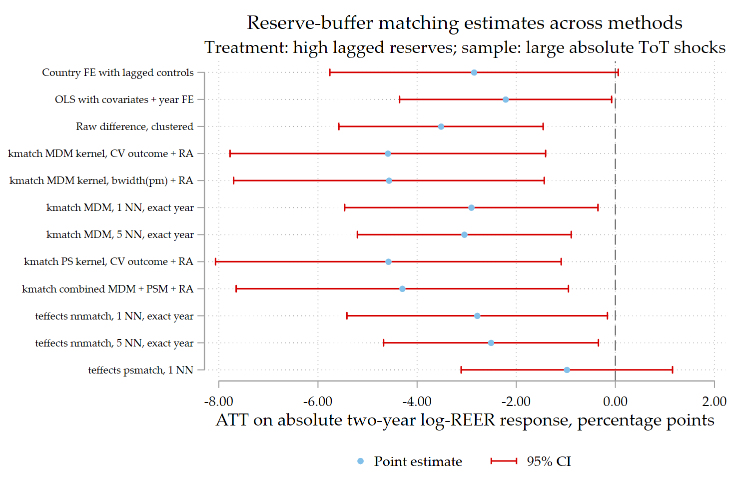
**Figure 1.** Reserve-buffer matching estimates across methods. Treatment is high lagged reserves; the sample is restricted to large absolute terms-of-trade shocks. The horizontal axis reports the ATT on the absolute two-year log-REER response in percentage points.

The figure is encouraging. Almost all estimators produce negative point estimates. The magnitude is economically meaningful: several estimates are around two to five percentage points. The consistency of the sign across raw, regression-adjusted, fixed-effect, nearest-neighbor, Mahalanobis-distance, propensity-score, and combined matching estimators suggests that the buffer pattern is not merely an artifact of one estimator.

The interpretation is straightforward: among country-years hit by large ToT disturbances, high-reserve observations tend to have a smaller absolute REER adjustment than comparable low-reserve observations.

7. Dynamic reserve-buffer effect

The next step is to check whether the result is dynamic. The outcome is recomputed at horizons h = 0, 1, 2, 3:

foreach h of numlist 0 1 2 3 {
    local yh "abs_cum_lreer_h`h'"
    kmatch ps high_res $X_PS ///
        (`yh' = $X_RA) ///
        if base_sample & large_absshock == 1 ///
           & !missing(high_res, `yh', abs_pre1, abs_pre2), ///
        att ematch(year) comsup bwidth(cv `yh') vce(cluster cn)
}

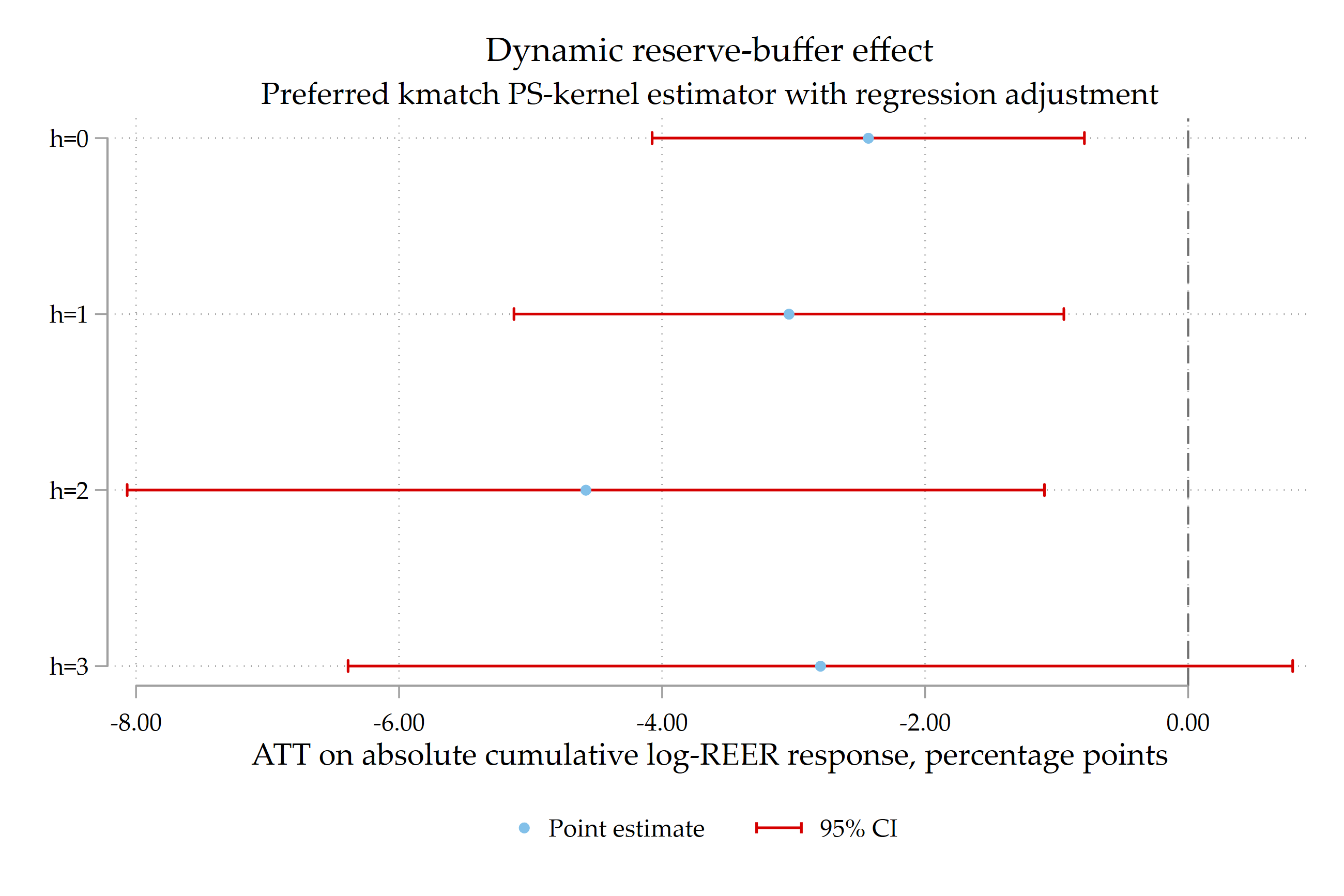
**Figure 2.** Dynamic reserve-buffer effect. The preferred `kmatch` propensity-score kernel estimator with regression adjustment is estimated separately for cumulative REER responses at horizons `h = 0, 1, 2, 3`.

The dynamic figure tells a coherent story. The buffer effect is negative at all horizons shown. It appears strongest around the two-year horizon, which is plausible for a real-exchange-rate adjustment mechanism. At longer horizons the confidence interval widens, so the result should be interpreted with caution rather than overstated.

Technical note. For a strict dynamic comparison, report the number of observations at each horizon. If the sample changes because future REER values are missing, a useful robustness check is to rerun the dynamic figure on the common sample for which all horizons h = 0, 1, 2, 3 are observed.

8. Placebo check

A useful placebo outcome is the absolute REER movement before the shock. If high-reserve countries were already following a systematically different REER path before the shock, the matching interpretation would be weaker.

* Placebo covariates exclude abs_pre1 because abs_pre1 is the placebo outcome.
global X_CORE_PLACEBO L1lreer abs_pre2 abs_Detot Detot shock_pos ///
                      L1lgdppk_m100 L1lgovexp L1irr L1ka_open L1lto L1fi
global X_RA_PLACEBO   $X_CORE_PLACEBO i.region_id

kmatch ps high_res $X_CORE_PLACEBO ///
    (abs_pre1 = $X_RA_PLACEBO) ///
    if match_sample, att ematch(year) comsup bwidth(cv abs_pre1) ///
    vce(cluster cn)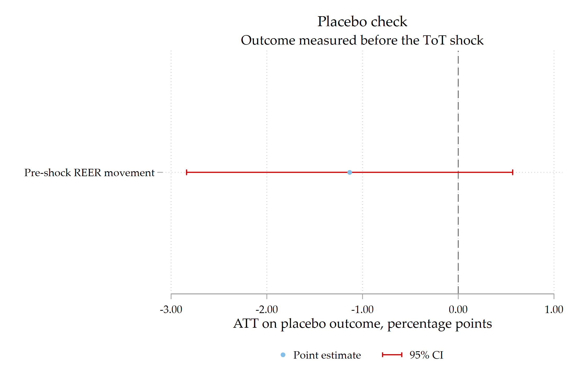

**Figure 3.** Placebo check. The outcome is the absolute REER movement before the ToT shock. A convincing buffer interpretation should not require a large and significant pre-shock difference.

The placebo estimate is imprecise and its confidence interval crosses zero. This is reassuring. The point estimate is not exactly zero, so the placebo should be reported honestly, but it does not show the same strong pattern as the post-shock outcomes.

9. Balance and common support

Matching estimates should not be reported without diagnostics. The credibility of the exercise depends on whether the matching procedure improves covariate balance and whether treated observations have comparable controls.

kmatch summarize
kmatch density, lw(*6 *2)
kmatch cumul, lw(*6 *2)
kmatch box
kmatch csummarize
kmatch cvplot, ms(o) index sort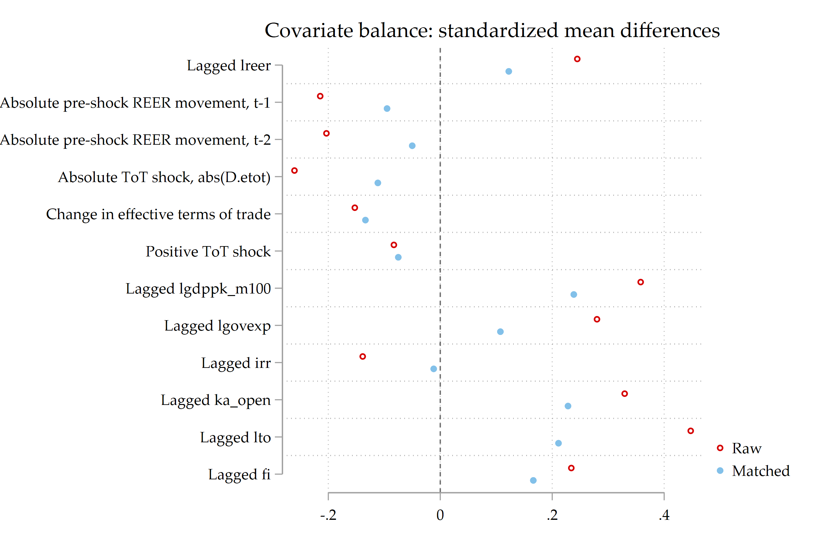

**Figure 4.** Covariate balance. Standardized mean differences before and after matching. The matched differences should be much closer to zero than the raw differences.

**Figure 5.** Propensity-score density before and after matching. The post-matching distributions should display improved overlap between treated and control observations.

These diagnostics are not cosmetic. If balance deteriorates after matching, the ATT is not credible. If common support is weak, the estimand applies only to the matched subset. The code therefore saves balance graphs, propensity-score density and cumulative distribution plots, box plots, common-support diagnostics, and the cross-validation bandwidth plot.

10. What is causal here?

The matching evidence is consistent with a reserve-buffer mechanism, but it should not be oversold as definitive causal proof. Matching adjusts for observed covariates. It does not eliminate unobserved confounding. Countries with high reserves may also differ in exchange-rate regimes, credibility, fiscal capacity, commodity exposure, financial depth, or policy reaction functions.

The most defensible claim is therefore:

Conditional on observed pre-shock characteristics and exposure to large ToT disturbances, high-reserve country-years experience smaller post-shock REER adjustments than comparable low-reserve country-years.

A stronger causal design would replace the observed ToT change with an external shift-share ToT shock based on predetermined trade weights and world commodity-price movements. It would also add threshold robustness, leave-one-region-out checks, and further pre-trend tests.

11. Robustness checks to add

Before treating the results as final, I would add four robustness checks.

Shock-threshold robustness: define large shocks using the 70th, 75th, and 80th percentiles of abs(D.etot).
Alternative reserve thresholds: compare the median split with a reserve-adequacy threshold, if available.
Leave-one-region-out estimates: check whether the result is driven by one region or one group of countries.
External ToT shocks: construct a shift-share shock using fixed trade weights and world price changes.

These extensions would move the exercise closer to a causal design. The matching framework would remain useful, but it would be embedded in a stronger identification strategy.

12. Conclusion

This application shows how matching can complement a panel interaction model. The original regression asks whether reserves moderate the relationship between terms of trade and the real exchange rate. The matching design translates that mechanism into a binary-treatment framework: after large ToT shocks, compare high-reserve observations with comparable low-reserve observations.

The results are encouraging. Across several estimators, high reserves are associated with a smaller absolute two-year REER response after large ToT shocks. The dynamic estimates suggest that the buffer effect is strongest around the two-year horizon, while the placebo outcome measured before the shock does not show a comparable significant effect.

The main lesson is methodological as well as economic. Matching is most useful when the estimand is aligned with the theory. In this case, the publishable matching question is not whether high terms of trade affect the REER. It is whether high reserves dampen the REER adjustment after large external disturbances.

Appendix: minimal Stata skeleton

* Packages
capture which moremata
if _rc ssc install moremata, replace
capture which kmatch
if _rc ssc install kmatch, replace
capture which coefplot
if _rc ssc install coefplot, replace

* Data
use datafintransformed-22-11-17.dta, clear
sort cn year
xtset cn year

* Region identifier
capture drop region_id
capture confirm numeric variable region
if !_rc {
    clonevar region_id = region
}
else {
    capture confirm variable regionname
    if !_rc egen region_id = group(regionname), label
    else egen region_id = group(countrycode), label
}

* Lags and shocks
foreach v in lreer lgdppk_m100 lgovexp irr ka_open lto fi lres etot {
    capture drop L1`v'
    gen double L1`v' = L.`v'
}

capture drop L2lreer L3lreer Detot abs_Detot abs_pre1 abs_pre2
gen double L2lreer   = L2.lreer
gen double L3lreer   = L3.lreer
gen double Detot     = D.etot
gen double abs_Detot = abs(Detot)
gen double abs_pre1  = abs(L1lreer - L2lreer)
gen double abs_pre2  = abs(L2lreer - L3lreer)

forvalues h = 0/3 {
    capture drop cum_lreer_h`h' abs_cum_lreer_h`h'
    if `h' == 0 gen double cum_lreer_h`h' = lreer - L1lreer
    else        gen double cum_lreer_h`h' = F`h'.lreer - L1lreer
    gen double abs_cum_lreer_h`h' = abs(cum_lreer_h`h')
}

* Conservative base sample
capture drop base_sample high_res large_absshock shock_pos match_sample
gen byte base_sample = (count_lgovexp == 20)
foreach v in lreer etot Detot abs_Detot L1lres L1lreer L2lreer L3lreer ///
             L1lgdppk_m100 L1lgovexp L1irr L1ka_open L1lto L1fi ///
             abs_pre1 abs_pre2 cn year region_id {
    replace base_sample = 0 if missing(`v')
}

* Treatment: high lagged reserves
bysort year: egen double med_L1lres = median(L1lres) if base_sample
gen byte high_res = (L1lres >= med_L1lres) if base_sample & !missing(L1lres, med_L1lres)

* Event: large absolute ToT shock
bysort year: egen double p75_abs_Detot = pctile(abs_Detot) if base_sample, p(75)
gen byte large_absshock = (abs_Detot >= p75_abs_Detot) if base_sample & !missing(abs_Detot, p75_abs_Detot)
gen byte shock_pos = (Detot > 0) if base_sample & !missing(Detot)

* Main matching sample
local yvar abs_cum_lreer_h2
gen byte match_sample = base_sample & large_absshock == 1 & ///
    !missing(high_res, `yvar', abs_pre1, abs_pre2)

* Covariates: do not include L1lres because it defines treatment
global X_CORE L1lreer abs_pre1 abs_pre2 abs_Detot Detot shock_pos ///
              L1lgdppk_m100 L1lgovexp L1irr L1ka_open L1lto L1fi

global X_PS $X_CORE
global X_RA $X_CORE i.region_id

* Preferred matching estimator
kmatch ps high_res $X_PS ///
    (`yvar' = $X_RA) ///
    if match_sample, att ematch(year) comsup bwidth(cv `yvar') ///
    vce(cluster cn)

* Diagnostics
kmatch summarize
kmatch density, lw(*6 *2)
kmatch cumul, lw(*6 *2)
kmatch box
kmatch csummarize
kmatch cvplot, ms(o) index sort

References

Aizenman, J., Ho, S. H., Huynh, L. D. T., Saadaoui, J., & Uddin, G. S. (2024). Real exchange rate and international reserves in the era of financial integration. Journal of International Money and Finance, 141, 103014.
Jann, Ben. 2017. “Kernel matching with automatic bandwidth selection.” London Stata Users Group Meeting.
Rosenbaum, Paul R., and Donald B. Rubin. 1983. “The Central Role of the Propensity Score in Observational Studies for Causal Effects.” Biometrika 70: 41–55.
Frölich, Markus. 2004. “Finite-sample properties of propensity-score matching and weighting estimators.” The Review of Economics and Statistics 86(1): 77–90.
Frölich, Markus. 2005. “Matching estimators and optimal bandwidth choice.” Statistics and Computing 15: 197–215.
Huber, Martin, Michael Lechner, and Conny Wunsch. 2013. “The performance of estimators based on the propensity score.” Journal of Econometrics 175: 1–21.
Huber, Martin, Michael Lechner, and Andreas Steinmayr. 2015. “Radius matching on the propensity score with bias adjustment: tuning parameters and finite sample behaviour.” Empirical Economics 49: 1–31.