Before reading this blog, I recommend you to read the first 3 parts of this blog series. Available below:
A narrative identification check: are the inflationary effects really causal?
A natural criticism of any recursive VAR is that the ordering assumption may be doing too much work. In the baseline panel VAR, country-specific geopolitical risk is ordered first, so the identifying assumption is that geopolitical risk does not react contemporaneously to macroeconomic conditions within the year. That is a plausible assumption, but it is still an assumption.
This is where Figure 6 becomes especially useful.
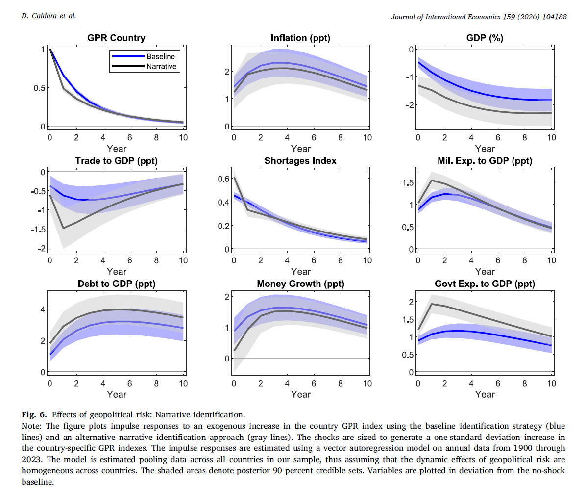
The point of the exercise is not to replace the baseline result. The point is to ask whether the baseline result survives when identification is tightened around a smaller set of large, plausibly exogenous geopolitical events. In the paper, the authors build a narrative geopolitical shock series by isolating country-year episodes in which geopolitical risk rises sharply for reasons that can be defended, historically, as not being driven by contemporaneous macroeconomic conditions. They then re-estimate the pooled panel VAR using that narrative shock as the driving innovation. The resulting impulse responses are compared with the baseline recursive specification.
The answer is clear: the core message survives.
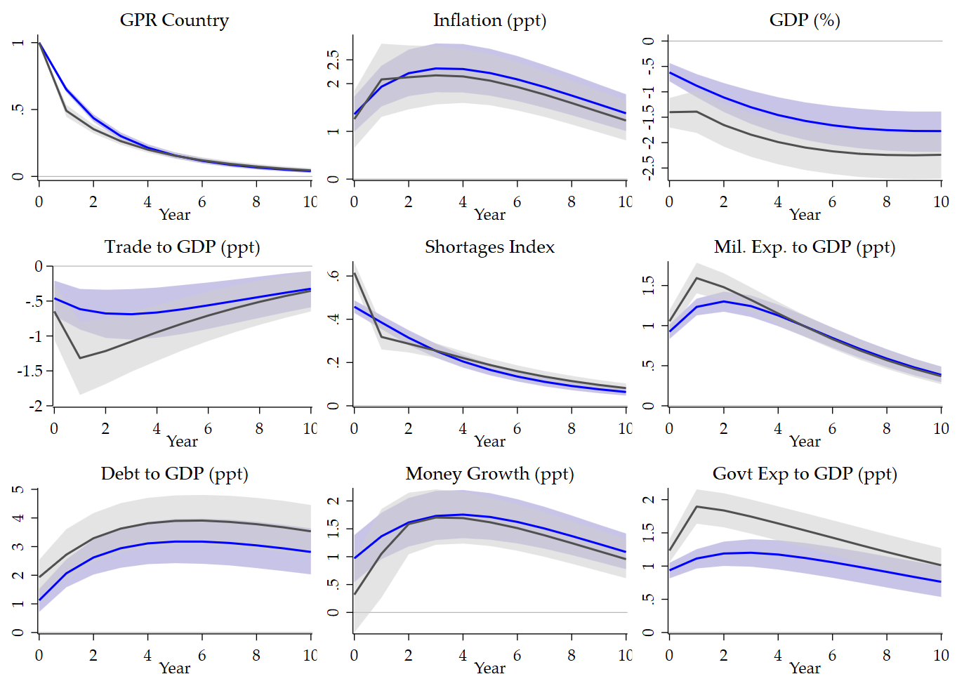
The replication figure:
Why this figure matters
By the time one reaches Figure 6, the baseline result is already established. Higher geopolitical risk raises inflation, lowers GDP, reduces trade, increases shortages, and is associated with more military spending, higher debt, faster money growth, and higher government spending. The concern, however, is always the same: perhaps some of these episodes reflect reverse causality, omitted contemporaneous forces, or broader macroeconomic distress that also happens to coincide with geopolitical turmoil.
Narrative identification is designed precisely to address that concern.
Instead of relying only on the Cholesky ordering, the approach starts from extreme country-specific GPR innovations, then checks whether those innovations correspond to historically identifiable geopolitical events that are plausibly orthogonal to domestic macroeconomic conditions. In other words, the narrative filter tries to separate true geopolitical shocks from episodes where economic distress may itself have been an important trigger.
That is why Figure 6 is so important. It asks whether the inflationary result is still there once we focus on large, historically validated geopolitical episodes.
What Figure 6 shows
The figure compares 2 sets of impulse responses:
- the baseline identification, in blue;
- the narrative identification, in gray.
The comparison is remarkably reassuring.
The first panel, for country GPR, already shows that the 2 shocks are very similar dynamically. Both generate a sharp increase on impact and then decay gradually over time. The narrative shock is a bit smaller after impact, but the overall persistence profile is close. This matters because it tells us that the alternative identification is not producing an entirely different shock process.
The second panel, for inflation, is the most important one. Inflation rises persistently under both identifications. The blue and gray median responses are extremely close: both rise for several years, both peak around the medium run, and both remain above baseline even after a decade. This is exactly what one would want from a robustness exercise. If the baseline inflation effect were an artifact of the recursive ordering, this is the place where it should fall apart. It does not.
The GDP panel tells a similar story. Output declines under both identifications. The narrative specification is even slightly more contractionary. So the stagflationary nature of the shock remains intact: higher inflation and lower activity still move together.
The same broad conclusion extends to the transmission channels.
Trade to GDP falls in both cases. The narrative response is initially more negative, which is intuitive: large geopolitical episodes often imply visible disruption to cross-border transactions, logistics, or commercial confidence.
The shortages index rises under both identifications, although the narrative response is somewhat front-loaded. Again, this is sensible. When the narrative method isolates large geopolitical episodes, it is likely selecting events with immediate and concrete disruptions.
Military expenditures, public debt, money growth, and government spending all move in the same qualitative direction under both approaches. The exact magnitudes differ, but the fiscal-monetary pattern remains the same. Geopolitical shocks are not just adverse news shocks. They are associated with a broader macroeconomic reallocation that includes defense spending, fiscal expansion, debt accumulation, and looser monetary conditions.
That consistency is the key result.
The economic interpretation
The narrative exercise strengthens the interpretation developed in the earlier figures.
The inflation response does not look like a standard demand boom. If it did, one would expect stronger activity, not a decline in GDP. Instead, the combination of higher inflation and weaker output points to a supply-disturbance logic, amplified by policy responses.
That mechanism is visible again here.
Trade falls. Shortages rise. GDP weakens. At the same time, governments react with higher spending and debt, while money growth also increases. The implication is not that every geopolitical shock works through exactly the same channel. Rather, the broad picture is that geopolitical disturbances tend to create scarcity, reallocation, and fiscal pressure, and these forces together make the shock inflationary.
Narrative identification matters because it tells us this interpretation is not merely a by-product of a recursive ordering convention. It survives when the shock series is rebuilt around historically identifiable events.
Why the match is not expected to be perfect
One should not expect the blue and gray lines to coincide exactly, and that is actually a good thing.
The baseline specification uses all observations and extracts innovations from the full reduced-form covariance structure. The narrative specification, by contrast, concentrates identification power in a subset of large events. It is therefore normal that some panels display somewhat different magnitudes. The narrative shock is a more selective object. It puts more weight on large, salient, and historically visible episodes.
What matters is that the qualitative pattern remains stable.
In fact, this is the right standard for a robustness exercise. Robustness does not mean identical numbers everywhere. It means that the central economic conclusion continues to hold under a stricter and conceptually different identification strategy.
That condition is clearly satisfied here.
What this adds to the replication narrative
For a replication blog series, this figure is especially valuable because it shows that the exercise is not only about matching shapes mechanically. It is also about understanding the econometric logic of the paper.
Figure 3 established the baseline pooled panel VAR result.
Figure 4 showed that both acts and threats matter, although acts tend to be stronger.
Figure 5 separated global from country-specific shocks.
Figure 6 then asks the most demanding question so far: are the baseline results still there once identification is pushed toward a narrative design built around large, plausibly exogenous geopolitical events?
The answer is yes.
That is why this figure works well as Part IV. It is a natural bridge between the baseline panel evidence and the later discussion of heterogeneity and spillovers. It tells the reader that the main result is not fragile. The inflationary effect of geopolitical risk is not just present in the preferred baseline model. It survives a demanding robustness check.
Bottom line
Figure 6 is one of the most persuasive figures in the paper.
It does not introduce a new headline result. Instead, it makes the existing headline result more credible. Inflation still rises. GDP still falls. Trade still contracts. Shortages still increase. Fiscal and monetary responses still move in the same broad direction.
So the main conclusion becomes harder to dismiss: geopolitical risk appears inflationary not only under a standard recursive identification, but also under a narrative strategy designed to isolate large, plausibly exogenous geopolitical events.
That is a strong result, and it is exactly the kind of robustness that gives the earlier figures more weight.
References
Caldara, D., Conlisk, S., Iacoviello, M., & Penn, M. (2026). Do geopolitical risks raise or lower inflation? Journal of International Economics, 104188.
Narrative identification
| Country | Year | Episode description | Included |
|---|---|---|---|
| Argentina | 1945 | War Declaration against Axis powers | Yes |
| Argentina | 1962 | Military coup against Frondizi (triggered by economic crisis and inflation) | No |
| Argentina | 1982 | Falklands War | Yes |
| Australia | 1941 | War mobilization against Japan | Yes |
| Australia | 1942 | Japanese attacks on Australia | Yes |
| Australia | 2022 | Ukraine war implications | Yes |
| Belgium | 1914 | German invasion (WWI) | Yes |
| Belgium | 1917 | Ongoing occupation | Yes |
| Belgium | 1940 | German invasion (WWII) | Yes |
| Brazil | 1930 | Revolution of 1930/Vargas coup | Yes |
| Brazil | 1942 | Brazil enters WWII | Yes |
| Brazil | 1962 | Involvement in the Cuban crisis | Yes |
| Canada | 1939 | Canada enters WWII | Yes |
| Canada | 1940 | Full war mobilization | Yes |
| Canada | 2022 | Ukraine war implications | Yes |
| Chile | 1914 | WWI | Yes |
| Chile | 1932 | Socialist Republic of Chile | Yes |
| Chile | 1973 | Pinochet coup against Allende (primarily driven by economic crisis) | No |
| China | 1950 | China enters Korean War | Yes |
| China | 1951 | Tibet annexation | Yes |
| China | 2022 | Taiwan tensions escalation | Yes |
| Colombia | 1901 | Thousand Days’ War peak (precipitated by coffee market collapse and depression) | No |
| Colombia | 1903 | Panama secedes from Colombia | Yes |
| Colombia | 1948 | Bogotazo riots/La Violencia begins (economic inequality as major contributing factor) | No |
| Denmark | 1917 | WWI submarine warfare impact | Yes |
| Denmark | 1939 | Pre-invasion neutrality crisis | Yes |
| Denmark | 1940 | German occupation | Yes |
| Egypt | 1956 | Suez Crisis | Yes |
| Egypt | 1967 | Six-Day War | Yes |
| Egypt | 1973 | Yom Kippur War | Yes |
| Finland | 1939 | Winter War begins | Yes |
| Finland | 1940 | Winter War major battles | Yes |
| Finland | 1944 | Soviet-Finnish War | Yes |
| France | 1914 | WWI begins | Yes |
| France | 1918 | German Spring Offensive | Yes |
| France | 1939 | WWII begins | Yes |
| Germany | 1914 | WWI begins | Yes |
| Germany | 1915 | Unrestricted submarine warfare | Yes |
| Germany | 1918 | German Revolution of 1918–1919 | Yes |
| Hong Kong | 1945 | Liberation from Japanese occupation | Yes |
| Hong Kong | 1967 | Riots during colonial rule | Yes |
| Hong Kong | 2019 | Pro-democracy protests | Yes |
| Hungary | 1914 | WWI mobilization | Yes |
| Hungary | 1944 | Nazi occupation | Yes |
| Hungary | 1956 | Hungarian Revolution | Yes |
| India | 1942 | Quit India Movement | Yes |
| India | 1944 | Bengal famine/Japanese threat | Yes |
| India | 1971 | Indo-Pakistani War/Bangladesh Liberation | Yes |
| Indonesia | 1942 | Japanese occupation begins | Yes |
| Indonesia | 1945 | Declaration of Independence | Yes |
| Indonesia | 1958 | PRRI-Permesta rebellion (regional economic grievances as possible driver) | No |
| Israel | 1967 | Six-Day War | Yes |
| Israel | 1973 | Yom Kippur War | Yes |
| Israel | 2023 | Hamas attack and Gaza war | Yes |
| Italy | 1935 | Ethiopian invasion | Yes |
| Italy | 1940 | Italy enters WWII | Yes |
| Italy | 1943 | Allied invasion/Mussolini ousted | Yes |
| Japan | 1904 | Russo-Japanese War begins | Yes |
| Japan | 1942 | Pacific War expansion | Yes |
| Japan | 1944 | Allied island-hopping campaign | Yes |
| Malaysia | 1941 | Japanese invasion begins | Yes |
| Malaysia | 1942 | Japanese occupation | Yes |
| Malaysia | 2014 | Flight MH370 disappearance (aviation incident without large geopolitical dimension) | No |
| Mexico | 1913 | Ten Tragic Days coup | Yes |
| Mexico | 1914 | US occupation of Veracruz | Yes |
| Mexico | 1916 | Pancho Villa raids/US expedition | Yes |
| Netherlands | 1914 | WWI neutrality crisis | Yes |
| Netherlands | 1939 | Pre-invasion mobilization | Yes |
| Netherlands | 1940 | German invasion | Yes |
| Norway | 1939 | Pre-invasion neutrality crisis | Yes |
| Norway | 1940 | German invasion | Yes |
| Norway | 1957 | NATO/Soviet tensions | Yes |
| Peru | 1933 | Colombian-Peruvian War | Yes |
| Peru | 2022 | Castillo coup attempt/impeachment (driven by economic grievances and inequality) | No |
| Peru | 2023 | Ongoing political instability (continuation of economic crisis from 2022) | No |
| Philippines | 1942 | Japanese invasion/occupation | Yes |
| Philippines | 1944 | Battle of Leyte Gulf | Yes |
| Philippines | 1945 | Liberation battle of Manila | Yes |
| Poland | 1939 | Nazi-Soviet invasion | Yes |
| Poland | 1944 | Warsaw Uprising | Yes |
| Poland | 2022 | Ukrainian refugee crisis | Yes |
| Portugal | 1936 | Spanish Civil War tensions | Yes |
| Portugal | 1961 | Colonial wars begin | Yes |
| Portugal | 1975 | Carnation Revolution aftermath | Yes |
| Russia | 1904 | Russo-Japanese War | Yes |
| Russia | 1914 | WWI begins | Yes |
| Russia | 2022 | Ukraine invasion | Yes |
| Saudi Arabia | 1990 | Gulf War threat from Iraq | Yes |
| Saudi Arabia | 2001 | 9/11 aftermath | Yes |
| Saudi Arabia | 2015 | Yemen intervention begins | Yes |
| South Africa | 1951 | Defiance Campaign begins | Yes |
| South Africa | 1976 | Soweto Uprising | Yes |
| South Africa | 1985 | State of Emergency declared (economic factors contributing to township unrest) | No |
| South Korea | 1950 | Korean War begins | Yes |
| South Korea | 1951 | Chinese intervention impact | Yes |
| South Korea | 2017 | North Korea missile crisis | Yes |
| Spain | 1914 | WWI neutrality pressures | Yes |
| Spain | 1936 | Spanish Civil War begins | Yes |
| Spain | 1937 | Spanish Civil War continuation | Yes |
| Sweden | 1939 | War preparations | Yes |
| Sweden | 1940 | Transit agreement with Nazi Germany | Yes |
| Sweden | 2022 | NATO application process due to war in Ukraine | Yes |
| Switzerland | 1918 | World War I | Yes |
| Switzerland | 1939 | War mobilization | Yes |
| Switzerland | 1940 | National Redoubt strategy | Yes |
| Taiwan | 1950 | US 7th Fleet deployments | Yes |
| Taiwan | 1955 | First Taiwan Strait Crisis | Yes |
| Taiwan | 1958 | Second Taiwan Strait Crisis | Yes |
| Thailand | 1941 | Japanese invasion | Yes |
| Thailand | 1972 | Student uprising (economic inequality as possible driver) | No |
| Thailand | 1975 | US military withdrawal | Yes |
| Tunisia | 1942 | WWII Tunisia Campaign begins | Yes |
| Tunisia | 1943 | Battle of Tunisia | Yes |
| Tunisia | 2011 | Jasmine Revolution | Yes |
| Turkey | 1912 | First Balkan War | Yes |
| Turkey | 1915 | Armenian Genocide | Yes |
| Turkey | 2022 | Military Tensions near border with Syria | Yes |
| Ukraine | 1918 | Independence declaration | Yes |
| Ukraine | 2014 | Crimea annexation/Donbas conflict | Yes |
| Ukraine | 2022 | Russian invasion | Yes |
| United Kingdom | 1914 | WWI begins | Yes |
| United Kingdom | 1915 | WWI escalation | Yes |
| United Kingdom | 1940 | Battle of Britain | Yes |
| United States | 2001 | 9/11 terrorist attacks | Yes |
| United States | 2022 | Ukraine war reaction/NATO mobilization | Yes |
| United States | 2023 | Chinese balloon incident/tensions | Yes |
| Venezuela | 1901 | Venezuelan Crisis beginning | Yes |
| Venezuela | 1902 | European naval blockade | Yes |
| Venezuela | 2019 | Presidential crisis (economic collapse as possible driver) | No |
| Vietnam | 1964 | Gulf of Tonkin incident | Yes |
| Vietnam | 1965 | US combat troops deployed | Yes |
| Vietnam | 1975 | Fall of Saigon | Yes |
Note: Listing of candidate narrative geopolitical shock episodes, indicating with “Yes” those included in the narrative index based on criteria excluding economic triggers.
Figure 5 code
version 18.0

capture log close _f6
log using "$JIE_LOG/23_figure6_narrative.log", replace text ///
    name(_f6)

use "$JIE_DER/annual_panel.dta", clear
sort country_id year
xtset country_id year

* ----------------------------------------------------------------------
* Baseline specification
* ----------------------------------------------------------------------
local yraw_base ///
    gpr_country ///
    inflation_ppt ///
    gdp_pct ///
    trade_to_gdp_ppt ///
    shortages_index ///
    milit_exp_to_gdp_ppt ///
    debt_to_gdp_ppt ///
    money_growth_ppt ///
    govt_exp_to_gdp_ppt

egen __rowmiss_f6b = rowmiss(`yraw_base')
gen byte sample_f6_base = (__rowmiss_f6b == 0)
drop __rowmiss_f6b

foreach v of local yraw_base {
    by country_id: egen mean_`v'_f6b = ///
        mean(cond(sample_f6_base, `v', .))
    gen dm_`v'_f6b = ///
        cond(sample_f6_base, `v' - mean_`v'_f6b, .)
}

local ydm_base
foreach v of local yraw_base {
    local ydm_base `ydm_base' dm_`v'_f6b
}

mata: jie_bvar_pooled_summary( ///
    "`ydm_base'", "country_id", "year", "sample_f6_base", ///
    $JIE_P, $JIE_H, $JIE_NDRAWS, 1, 1, ///
    "F6B_Q05", "F6B_Q50", "F6B_Q95", ///
    "F6B_MEAN", "F6B_VAR", "F6B_Neff" ///
)

* ----------------------------------------------------------------------
* Narrative specification
* ----------------------------------------------------------------------
local yraw_narr ///
    gpr_narrative ///
    gpr_country ///
    inflation_ppt ///
    gdp_pct ///
    trade_to_gdp_ppt ///
    shortages_index ///
    milit_exp_to_gdp_ppt ///
    debt_to_gdp_ppt ///
    money_growth_ppt ///
    govt_exp_to_gdp_ppt

egen __rowmiss_f6n = rowmiss(`yraw_narr')
gen byte sample_f6_narr = (__rowmiss_f6n == 0)
drop __rowmiss_f6n

foreach v of local yraw_narr {
    by country_id: egen mean_`v'_f6n = ///
        mean(cond(sample_f6_narr, `v', .))
    gen dm_`v'_f6n = ///
        cond(sample_f6_narr, `v' - mean_`v'_f6n, .)
}

local ydm_narr
foreach v of local yraw_narr {
    local ydm_narr `ydm_narr' dm_`v'_f6n
}

mata: jie_bvar_pooled_summary( ///
    "`ydm_narr'", "country_id", "year", "sample_f6_narr", ///
    $JIE_P, $JIE_H, $JIE_NDRAWS, 1, 2, ///
    "F6N_Q05", "F6N_Q50", "F6N_Q95", ///
    "F6N_MEAN", "F6N_VAR", "F6N_Neff" ///
)

display as text "Figure 6 baseline lag-valid pooled rows: " ///
    %9.0g scalar(F6B_Neff)

display as text "Figure 6 narrative lag-valid pooled rows: " ///
    %9.0g scalar(F6N_Neff)

* Keep narrative responses for cols 2..10 so displayed variables match Fig. 3
matrix F6N_Q05P = F6N_Q05[1..rowsof(F6N_Q05), 2..colsof(F6N_Q05)]
matrix F6N_Q50P = F6N_Q50[1..rowsof(F6N_Q50), 2..colsof(F6N_Q50)]
matrix F6N_Q95P = F6N_Q95[1..rowsof(F6N_Q95), 2..colsof(F6N_Q95)]

local cnB05
local cnB50
local cnB95
local cnN05
local cnN50
local cnN95

foreach v of local yraw_base {
    local cnB05 `cnB05' base_q05_`v'
    local cnB50 `cnB50' base_q50_`v'
    local cnB95 `cnB95' base_q95_`v'
    local cnN05 `cnN05' narr_q05_`v'
    local cnN50 `cnN50' narr_q50_`v'
    local cnN95 `cnN95' narr_q95_`v'
}

matrix colnames F6B_Q05  = `cnB05'
matrix colnames F6B_Q50  = `cnB50'
matrix colnames F6B_Q95  = `cnB95'
matrix colnames F6N_Q05P = `cnN05'
matrix colnames F6N_Q50P = `cnN50'
matrix colnames F6N_Q95P = `cnN95'

preserve
clear
set obs `= $JIE_H + 1'
gen horizon = _n - 1

svmat double F6B_Q05,  names(col)
svmat double F6B_Q50,  names(col)
svmat double F6B_Q95,  names(col)
svmat double F6N_Q05P, names(col)
svmat double F6N_Q50P, names(col)
svmat double F6N_Q95P, names(col)

* Match Figure 3 scaling for GDP
replace base_q05_gdp_pct = 100 * base_q05_gdp_pct
replace base_q50_gdp_pct = 100 * base_q50_gdp_pct
replace base_q95_gdp_pct = 100 * base_q95_gdp_pct

replace narr_q05_gdp_pct = 100 * narr_q05_gdp_pct
replace narr_q50_gdp_pct = 100 * narr_q50_gdp_pct
replace narr_q95_gdp_pct = 100 * narr_q95_gdp_pct

save "$JIE_DER/fig6_irf.dta", replace
export delimited using "$JIE_DER/fig6_irf.csv", replace

local gtitle_gpr_country          "GPR Country"
local gtitle_inflation_ppt        "Inflation (ppt)"
local gtitle_gdp_pct              "GDP (%)"
local gtitle_trade_to_gdp_ppt     "Trade to GDP (ppt)"
local gtitle_shortages_index      "Shortages Index"
local gtitle_milit_exp_to_gdp_ppt "Mil. Exp. to GDP (ppt)"
local gtitle_debt_to_gdp_ppt      "Debt to GDP (ppt)"
local gtitle_money_growth_ppt     "Money Growth (ppt)"
local gtitle_govt_exp_to_gdp_ppt  "Govt Exp to GDP (ppt)"

* Use Figure 3 journal-style axis settings
local yset_gpr_country ///
    "yscale(range(-0.02 1.05)) ylabel(0 .5 1, nogrid labsize(medsmall))"

local yset_inflation_ppt ///
    "yscale(range(0 3)) ylabel(0 1 2 2.5, nogrid labsize(medsmall))"

local yset_gdp_pct ///
    "yscale(range(-2.3 0.1)) ylabel(-2.5 -2 -1.5 -1 -.5 0, nogrid labsize(medsmall))"

local yset_trade_to_gdp_ppt ///
    "yscale(range(-1.15 0.05) noextend) ylabel(-2 -1.5 -1 -.5 0, angle(horizontal) nogrid labsize(medsmall))"

local yset_shortages_index ///
    "yscale(range(0 .5)) ylabel(0 .2 .4 .6, nogrid labsize(medsmall))"

local yset_milit_exp_to_gdp_ppt ///
    "yscale(range(0 1.4)) ylabel(0 .5 1 1.5, nogrid labsize(medsmall))"

local yset_debt_to_gdp_ppt ///
    "yscale(range(0 4.2)) ylabel(0 1 2 3 4 5, nogrid labsize(medsmall))"

local yset_money_growth_ppt ///
    "yscale(range(0 2.2)) ylabel(0 .5 1 1.5 2, nogrid labsize(medsmall))"

local yset_govt_exp_to_gdp_ppt ///
    "yscale(range(0 1.4)) ylabel(0 .5 1 1.5 2, nogrid labsize(medsmall))"

local base_line  "blue"
local base_band  "lavender"
local narr_line  "gs5"
local narr_band  "gs12"

local graphs
local i = 0

foreach v of local yraw_base {
    local ++i

    if `i' == 1 {
        local legopt ///
            legend(off)
    }
    else {
        local legopt legend(off)
    }

    twoway ///
        rarea base_q05_`v' base_q95_`v' horizon, ///
            color(`base_band'%65) lcolor(`base_band'%0) || ///
        rarea narr_q05_`v' narr_q95_`v' horizon, ///
            color(`narr_band'%55) lcolor(`narr_band'%0) || ///
        line base_q50_`v' horizon, ///
            lcolor(`base_line') lwidth(medthick) || ///
        line narr_q50_`v' horizon, ///
            lcolor(`narr_line') lwidth(medthick) || ///
        , ///
        title("`gtitle_`v''", size(medium) color(black)) ///
        yline(0, lcolor(black%35) lwidth(vthin)) ///
        xtitle("Year", size(medsmall)) ///
        ytitle("") ///
        xlabel(0(2)$JIE_H, labsize(medsmall) nogrid) ///
        `yset_`v'' ///
        `legopt' ///
        graphregion(color(white) margin(small)) ///
        plotregion(color(white) margin(tiny)) ///
        name(gr6_`v', replace)

    local graphs `graphs' gr6_`v'
}

graph combine `graphs', ///
    cols(3) ///
    imargin(1 1 1 1) ///
    graphregion(color(white) margin(2 2 2 2)) ///
    name(fig6_combined, replace)

graph save "$JIE_FIG/figure6_narrative_journalstyle.gph", replace
graph export "$JIE_FIG/figure6_narrative_journalstyle.png", ///
    width(2400) replace

restore
log close _f6