Drawing Local Projection IRFs with Driscoll-Kraay Inference in Stata

Local projections (LPs) have become a workhorse tool in applied macroeconomics since Jordà (2005). They are flexible, robust to misspecification, and easy to interpret. In panel settings, however, inference can be delicate. Especially when shocks are common across cross-sectional units, as is often the case with monetary, geopolitical, or global shocks.

This post explains how to construct LP impulse response functions (IRFs) using Driscoll-Kraay (DK) standard errors in Stata, relying on the xtscc command.

1. Why combine LPs and Driscoll-Kraay?

In panel LPs of the form

$$y_{i,t+h}=\alpha_{i,h}+\beta_h \varepsilon_t+\sum_{j=1}^{p}\Gamma_{h,j}X_{i,t-j}+u_{i,t+h}, \qquad h=0,1,\dots,H.$$$$

the shock $\varepsilon_t$​ is often common across units (e.g. a global geopolitical shock). This induces cross-sectional dependence in the error term. Standard clustering at the unit level may understate uncertainty.

Driscoll–Kraay standard errors are designed precisely for this situation:

• robust to heteroskedasticity,
• robust to serial correlation,
• robust to cross-sectional dependence when $T$ is moderate.

They are conservative. But that is a feature, not a bug, when shocks are common.

2. Why xtscc instead of locproj?

The locproj command is ideal for baseline LP estimation and visualization. However, it does not implement Driscoll–Kraay standard errors.

The workaround is simple:

• LPs are just separate regressions for each horizon.
• We can estimate each horizon with xtscc,
• collect coefficients and standard errors,
• and then reconstruct the IRF by hand.

This is precisely what we do below.

3. Step 1: Set up the panel and horizons

xtset unit_id period
local H 2

Assume:

• D.GDP is growth (Δ log GDP),
• z_D_LUSA is a standardized common shock (e.g. US–China relations),
• controls are lagged macro variables.

4. Step 2: Create horizon-specific outcomes

Local projections regress future outcomes on today’s shock. For each horizon $h$h:

forvalues h = 0/`H' {
    gen double y`h' = F`h'.D.GDP
}

Now y0, y1, y2 correspond to horizons 0, 1, and 2.

5. Step 3: Estimate LPs with Driscoll-Kraay SEs

For each horizon, run a DK regression:

xtscc y`h' z_D_LUSA ///
    L(1/2).(CPI TRADE GFCF POP TOT) L(1/2).D.GDP, fe

This gives:

• the horizon-$h$ response $\hat\beta_h$​,
• Driscoll–Kraay standard errors,
• appropriate degrees of freedom.

You then post these estimates into a temporary dataset.

That block is the “data engineering” step that turns a sequence of horizon-by-horizon regressions into a dataset you can plot. Here is what each line is doing and why it is needed.

You are estimating, for each horizon $h$, one regression and obtaining one coefficient $\hat\beta_h$ (plus its DK standard error). To draw an IRF, you require a table like:

$$(h,\ \hat\beta_h,\ \widehat{se}_h,\ df_h) \quad \text{for } h=0,\dots,H.$$

Stata does not automatically build that table. The postfile machinery does.

---

A1) Temporary “handles” and file names

tempname posth
tempfile irfdk

• tempname posth creates a temporary name for a Stata “posting handle.” Think of it as a pointer to a file you will be writing rows into.
• tempfile irfdk creates a temporary filename on disk (something like C:\...\ST_XXXX.tmp) that will store the posted dataset. You do not need to manage the path; Stata does it.

A2) Initialize an empty dataset to store results

postfile `posth' int h double b se df using `irfdk', replace

This creates an empty dataset (at irfdk) with 4 variables:

• h (integer): the horizon (0, 1, 2, …)
• b (double): the coefficient $\hat\beta_h$​ on the shock at horizon⁣ $h$
• se (double): the Driscoll–Kraay standard error for that coefficient
• df (double): residual degrees of freedom used for the $t$-critical values (needed to form CIs)

The option replace overwrites any existing temporary file with the same name (safe here because it is a tempfile).

A3) Loop over horizons and “post” one row per regression

forvalues h = 0/`H' {
    xtscc y`h' `shock' `X', fe
    scalar b  = _b[`shock']
    scalar se = _se[`shock']
    scalar df = e(df_r)
    post `posth' (`h') (b) (se) (df)
}

Step by step:

1. xtscc yh'shock' `X', fe
   runs the horizon-$h$ LP regression with Driscoll–Kraay SEs.
2. scalar b = _b[`shock'] extracts the estimated coefficient on the shock._b[varname]` is Stata’s stored coefficient for the last estimation.
3. scalar se = _se[`shock'] extracts the standard error for that same coefficient. With xtscc, this is the DK standard error.
4. scalar df = e(df_r)
   stores the residual degrees of freedom from the regression. DK inference uses $t$t-statistics, so you need df to compute correct critical values via invttail().
5. post `posth' (`h') (b) (se) (df)
   appends a new row to the posted dataset with:
   • the horizon index h
   • the coefficient b
   • the standard error se
   • df df

After the loop finishes, you have $H+1$ rows: one per horizon.

A4) Close the posting file (important)

postclose `posth'

This finalizes the dataset on disk. If you forget this, Stata may not write the rows properly, and use irfdk', clear can fail or load an incomplete dataset.

A5) Load the results dataset and order horizons

use `irfdk', clear
sort h

• use irfdk’, clear` loads the dataset you just created (one row per horizon).
• sort h ensures horizons are in ascending order so that twoway rarea and line connect points correctly.

At this point, you are ready to compute confidence intervals (lo95, hi95, etc.) and plot.

Practical note

This approach is robust and general: you can store additional objects the same way (p-values, N, R²) by adding more columns to the postfile line and posting them inside the loop.

---

6. Step 4: Build confidence intervals

Because DK uses $t$t-statistics, confidence intervals should be based on the Student-t distribution, not normal quantiles.

For example:

gen t95 = invttail(df, 0.025)
gen t90 = invttail(df, 0.05)
gen t68 = invttail(df, 0.16)

gen double lo95 = b - t95*se
gen double hi95 = b + t95*se
gen double lo90 = b - t90*se
gen double hi90 = b + t90*se
gen double lo68 = b - t68*se
gen double hi68 = b + t68*se

7. Step 5: Plot the IRF

Finally, reconstruct the IRF using twoway:

twoway ///
    (rarea hi95 lo95 h, fcolor(gs14%20) lcolor(none)) ///
    (rarea hi90 lo90 h, fcolor(gs12%30) lcolor(none)) ///
    (rarea hi68 lo68 h, fcolor(gs10%40) lcolor(none)) ///
    (line b h, lcolor(black) lwidth(medthick)) ///
    , yline(0, lcolor(black%40)) ///
      xlabel(0 1 2) xscale(range(0 2)) ///
      xtitle("Horizon") ///
      ytitle("Response of GDP growth") ///
      graphregion(color(white))

This produces a publication-quality DK–LP IRF with layered confidence bands.

8. How to interpret DK–LP IRFs

A key point: DK inference is conservative.

• If an effect survives DK, it is genuinely robust.
• If it disappears, this does not mean the effect is zero, only that it is imprecisely estimated once cross-sectional dependence is fully accounted for.

In practice:

• Use standard LPs with clustered SEs as your baseline.
• Use DK–LP IRFs as strict robustness checks.

This is now standard practice in applied macro and regional economics.

9. Takeaways

• LPs and Driscoll–Kraay inference are fully compatible.
• xtscc allows you to handle common shocks cleanly.
• DK–LP IRFs are ideal for robustness, not necessarily for baseline storytelling.
• With⁣ $T \approx 20$ and common shocks, conservative inference is the right choice.

Final thought

If your results weaken under DK but keep their sign and economic logic, that is good econometrics, not a failure. You are learning where the signal is strong, and where it is not.

This is precisely what empirical macroeconomics should do.

Full code below:

**# Set the directory

cd C:\Users\jamel\Dropbox\Latex\PROJECTS\

cd 26-01-china-growth-geopolitics-provinces

**# Import the data from Tsinghua University

import excel "Dataset.xlsx", sheet("Feuil1") firstrow clear

generate Period = tm(1950m1) + _n-1
format %tm Period

tsset Period

keep if Period>=tm(1990m1)

set varabbrev off

gen year = yofd(A)

format %ty year

**# Switch from annual to monthly frequency (accumulate)

collapse (mean) USA JPN RUS UK FRA INDIA GER VN CDS AUS INDO PAK, by(year)

tsset year

**# Create the log-modulus transformation and the difference of it

foreach v in JPN AUS FRA GER UK USA ///
 INDO PAK RUS VN INDIA CDS{
 	/* Another transformation for the PRI index */
    gen L`v' = sign(`v') * log(1 + abs(`v'))
	gen DL`v' = d.L`v'
 }

label variable LJPN "PRI Japan-China"
label variable LAUS "PRI Australia-China"
label variable LCDS "PRI South Korea-China"
label variable LFRA "PRI France-China"
label variable LGER "PRI Germany-China"
label variable LINDIA "PRI India-China"
label variable LINDO "PRI Indonesia-China"
label variable LPAK "PRI Pakistan-China"
label variable LRUS "PRI Russia-China"
label variable LVN "PRI Vietnam-China"
label variable LUK "PRI United Kingdom-China" 
label variable LUSA "PRI US-China"

tsline L*, xscale(range(1990 2024)) ///
 xlabel(1990(4)2024) name(Fig1, replace)
 
graph export Fig1.png, as(png) width(3000) replace

save data_pri_annual.dta, replace

**# Merge with provincial data

merge m:m year using ///
dataset_provinces_with_political_turnover.dta           

tsfill, full

xtset unit_id year

xtdes

**# Local Projections

rename (g2_gdppc_const05_new ///
 slog_cpi_new ln_trade_share_new ///
 ln_gfcf_share_new g2_pop_new g2_tot_new) ///
 (GDPPC ///
 CPI TRADE ///
 GFCF POP TOT)

eststo m1: reghdfe GDPPC L.GDPPC ///
 L.CPI L.TRADE ///
 L.GFCF L.POP L.TOT, ///
 a(year unit_id) vce(cluster unit_id)

eststo m2: xtdpdbc GDPPC ///
 L.CPI L.TRADE ///
 L.GFCF L.POP L.TOT, ///
 fe vce(r) teffects
 
eststo m3: xtscc GDPPC ///
 L.GDPPC ///
 L.CPI L.TRADE ///
 L.GFCF L.POP L.TOT, fe
 
esttab m*, se stats(r2 N F, fmt(%7.2f)) ///
 star(* 0.10 ** 0.05 *** 0.01) b(%7.4f) ///
 keep(L.GDPPC ///
 L.CPI L.TRADE ///
 L.GFCF L.POP L.TOT)

sort unit_id year
by unit_id: gen period = 1990 + _n - 1
drop if unit_id==.

xtset unit_id period

order unit_id period

/// if you want use Newey-West you need a balanced panel

gen GDP = log(gdp_new)

summ D.GDP D.LUSA D.LJPN D.LINDIA

*------------------------------------------------------------
* Standardize the shocks in the same form used in LP: D.L*
*------------------------------------------------------------

* US-China
summ D.LUSA if !missing(D.LUSA)
gen z_D_LUSA = (D.LUSA - r(mean))/r(sd)

* China-Japan
summ D.LJPN if !missing(D.LJPN)
gen z_D_LJPN = (D.LJPN - r(mean))/r(sd)

* China-India
summ D.LINDIA if !missing(D.LINDIA)
gen z_D_LINDIA = (D.LINDIA - r(mean))/r(sd)

locproj D.GDP, shock(z_D_LUSA) ///
    h(2) yl(2) sl(0) zero ///
    c(L(1/2).(CPI TRADE GFCF POP TOT)) fe ///
    conf(90 95) vce(cluster unit_id) ///
    ttitle("Horizon") title(`"US-China"') ///
    noisily stats save irfname(iUS) grname(US) margins

locproj D.GDP, shock(z_D_LJPN) ///
    h(2) yl(2) sl(0) zero  ///
    c(L(1/2).(CPI TRADE GFCF POP TOT)) fe ///
    conf(90 95) vce(cluster unit_id) ///
    ttitle("Horizon") title(`"China-Japan"') ///
    noisily stats save irfname(iJPN) grname(JPN)

locproj D.GDP, shock(z_D_LINDIA) ///
    h(2) yl(2) sl(0) zero ///
    c(L(1/2).(CPI TRADE GFCF POP TOT)) fe ///
    conf(90 95) vce(cluster unit_id) ///
    ttitle("Horizon") title(`"China-India"') ///
    noisily stats save irfname(iINDIA) grname(INDIA)

*------------------------------------------------------------
* DK-LP (xtscc) IRF graph for horizons h=0..H
*------------------------------------------------------------

cls

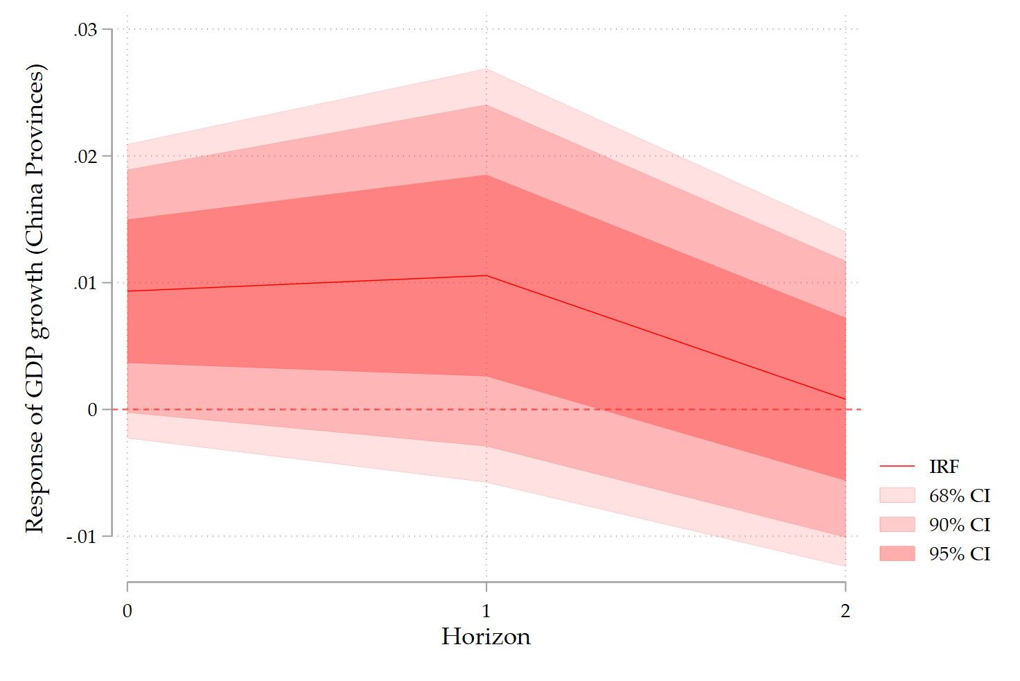
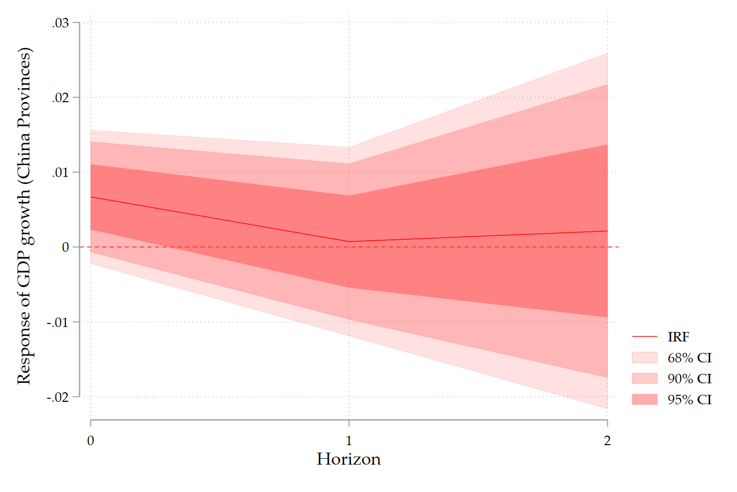
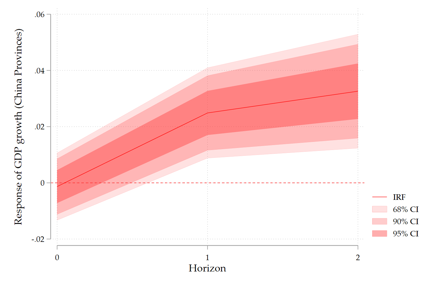
foreach v in z_D_LUSA z_D_LJPN z_D_LINDIA {

preserve

	* Panel declaration
	xtset unit_id period

	* Choose shock and horizon
	local shock   "`v'"   // or z_D_LJPN, z_D_LINDIA, etc.
	local H       2            // max horizon

	* Controls (match what you used in the DK regressions)
	local X "L(1/2).(CPI TRADE GFCF POP TOT) L(1/2).D.GDP"

	* Create horizon outcomes y_h = F^h D.GDP
	forvalues h = 0/`H' {
		capture drop y`h'
		gen double y`h' = F`h'.D.GDP
	}

	* Collect DK coefficients and SEs
	tempname posth
	tempfile irfdk
	postfile `posth' int h double b se df using `irfdk', replace

	forvalues h = 0/`H' {
		xtscc y`h' `shock' `X', fe
		scalar b  = _b[`shock']
		scalar se = _se[`shock']
		scalar df = e(df_r)
		post `posth' (`h') (b) (se) (df)
	}
	postclose `posth'

	use `irfdk', clear
	sort h

	* Build 90% and 95% CIs using t critical values
	gen double t95 = invttail(df, 0.025)
	gen double t90 = invttail(df, 0.05)
	gen double t68 = invttail(df, 0.16)

	gen double lo95 = b - t95*se
	gen double hi95 = b + t95*se
	gen double lo90 = b - t90*se
	gen double hi90 = b + t90*se
	gen double lo68 = b - t68*se
	gen double hi68 = b + t68*se

	twoway ///
		(rarea hi68 lo68 h, sort fcolor(red%40) lcolor(red) ///
		lwidth(vvthin)) ///
		(rarea hi90 lo90 h, sort fcolor(red%25) lcolor(red) ///
		lwidth(vvthin)) ///
		(rarea hi95 lo95 h, sort fcolor(red%15) lcolor(red) ///
		lwidth(vvthin)) ///
		(line b h, sort lcolor(red) lwidth(vthin)) ///
		, yline(0, lcolor(red%60)) ///
		  xlabel(0 1 2) ///
                  xscale(range(0 2)) ///
		  xtitle("Horizon") ///
		  ytitle("Response of GDP growth (China Provinces)") ///
		  legend(order(4 "IRF" 3 "68% CI" 2 "90% CI" 1 "95% CI")) ///
		  graphregion(color(white)) ///
		  plotregion(color(white)) name(G`v', replace)

restore

}